Unit outcomes

By the end of this unit you will be able to:

• Determine the domain and range of exponential functions of the form [latex]\scriptsize y=a.{{b}^{{x+p}}}+q,b \gt 0[/latex].
• Find the asymptote of exponential functions of the form [latex]\scriptsize y=a.{{b}^{{x+p}}}+q,b \gt 0[/latex].
• Find the intercepts with the axes of exponential functions of the form [latex]\scriptsize y=a.{{b}^{{x+p}}}+q,b \gt 0[/latex].
• Sketch exponential functions of the form [latex]\scriptsize y=a.{{b}^{{x+p}}}+q,b \gt 0[/latex].

What you should know

Before you start this unit, make sure you can:

• Solve exponential equations.
• Plot exponential functions of the form [latex]\scriptsize y=a.{{b}^{x}}+q[/latex].
• Determine the x- and y-intercepts of exponential functions of the form [latex]\scriptsize y=a.{{b}^{x}}+q[/latex].
• Determine the domain and range of exponential functions of the form [latex]\scriptsize y=a.{{b}^{x}}+q[/latex].
• Determine the asymptote of exponential functions of the form [latex]\scriptsize y=a.{{b}^{x}}+q[/latex].

Refer to level 2 subject outcome 2.1 unit 4 if you require assistance with any of these skills.

Introduction

In level 2 we were introduced to the exponential function of the form [latex]\scriptsize y=a.{{b}^{x}}+q,b \gt 0[/latex]. We learnt that the term ‘exponential growth’ is sometimes used to refer to something that happens very quickly. We also learnt that in Mathematics ‘exponential’ has a very specific meaning and exponential functions are specific kinds of functions.

We saw that there are many processes in nature and finance where the relationship between the inputs and outputs is exponential. One example is how bacteria reproduce. Bacteria reproduce by simply splitting into two new bacteria. If one bacterium splits into two and then each of these splits into two and then each of these splits into two, etc. pretty soon we have a whole lot of bacteria!

We learnt that these functions behave quite similarly to the other functions we have explored so far. Therefore, much of what we already know about linear, quadratic and hyperbolic functions can be applied to exponential functions as well.

Take note!

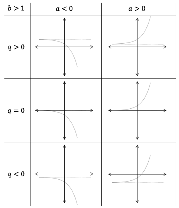
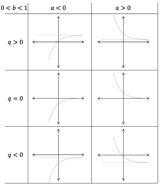
The effect of [latex]\scriptsize a[/latex] and [latex]\scriptsize b[/latex]:

if [latex]\scriptsize b \gt 1[/latex], the function value increases to positive infinity (if [latex]\scriptsize a \gt 1[/latex]) or negative infinity (if [latex]\scriptsize a \lt 1[/latex]) as [latex]\scriptsize x[/latex] increases

if [latex]\scriptsize 0 \lt b \lt 1[/latex], the function value increases to positive infinity (if [latex]\scriptsize a \gt 1[/latex]) or negative infinity (if [latex]\scriptsize a \lt 1[/latex]) as [latex]\scriptsize x[/latex] decreases.

The effect of [latex]\scriptsize q[/latex]:

if [latex]\scriptsize q \gt 0[/latex], the function is shifted up by [latex]\scriptsize q[/latex] units

if [latex]\scriptsize q \lt 0[/latex], the function is shifted down by [latex]\scriptsize q[/latex] units

Horizontal asymptote is the line [latex]\scriptsize y=q[/latex].

If [latex]\scriptsize a \gt 1[/latex], the graph lies above the asymptote.

If [latex]\scriptsize a \lt 1[/latex], the graph lies below the asymptote.

Note: It is important to remember that the value of [latex]\scriptsize b[/latex] must be greater than zero. Negatives of [latex]\scriptsize b[/latex] do not produce a continuous graph.

The exponential function of the form [latex]\scriptsize y=a.{{b}^{{x+p}}}+q,b \gt 0[/latex]

We know that the value of [latex]\scriptsize q[/latex] in [latex]\scriptsize y=a.{{b}^{x}}+q[/latex] shifts the graph vertically up or down. Now, let’s investigate the effect of [latex]\scriptsize p[/latex] in [latex]\scriptsize y=a.{{b}^{{x+p}}}+q[/latex]. Based on your knowledge of the effect of [latex]\scriptsize p[/latex] in the turning point form of the quadratic function [latex]\scriptsize y=a{{(x+p)}^{2}}+q[/latex], and the hyperbolic function [latex]\scriptsize y=\displaystyle \frac{a}{{x+p}}+q[/latex], what do you think this effect will be?

Figure 3 shows the graphs of three exponential functions, [latex]\scriptsize f(x)=1\times {{2}^{x}}[/latex], [latex]\scriptsize g(x)=1\times {{2}^{{(x+2)}}}[/latex] and [latex]\scriptsize h(x)=1\times {{2}^{{(x-3)}}}[/latex]. We can see that because [latex]\scriptsize a \gt 0[/latex] and [latex]\scriptsize b \gt 1[/latex] in each case, all three functions increase in value as [latex]\scriptsize x[/latex] increases. Because [latex]\scriptsize q=0[/latex], all three functions have a horizontal asymptote of [latex]\scriptsize y=0[/latex] or the x-axis.

But what is different? Have a look at the various points that have been labelled on each graph. Can you see the difference between the points with the same y-coordinates? What is this difference and how does this difference relate to the equation of each function?

We can see that the point [latex]\scriptsize (0,1)[/latex] on [latex]\scriptsize f(x)[/latex] has been shifted two units to the left and is now the point [latex]\scriptsize (-2,1)[/latex] on [latex]\scriptsize g(x)[/latex]. This same point on [latex]\scriptsize f(x)[/latex] has been shifted three units to the right and is now the point [latex]\scriptsize (3,1)[/latex] on [latex]\scriptsize h(x)[/latex].

The same horizontal shifting pattern can be seen for the points [latex]\scriptsize (1,2)[/latex] and [latex]\scriptsize (2,4)[/latex] on [latex]\scriptsize f(x)[/latex]. These are shifted two units to the left on [latex]\scriptsize g(x)[/latex] and three units to the right on [latex]\scriptsize h(x)[/latex].

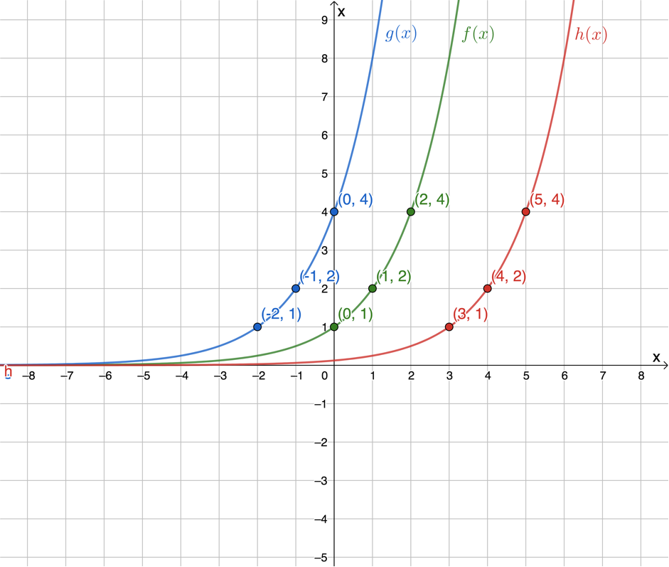
Therefore, the effect of [latex]\scriptsize p[/latex] on the function [latex]\scriptsize y=a.{{b}^{{x+p}}}+q,b \gt 0[/latex] is a horizontal shift because all the points on the graph are moved the same distance in the same direction. In other words, the entire graph shifts to the left or to the right.

• If [latex]\scriptsize p \gt 0[/latex] the graph is shifted [latex]\scriptsize p[/latex] units to the left.
• If [latex]\scriptsize p \lt 0[/latex] the graph is shifted [latex]\scriptsize p[/latex] units to the right.

Domain and range of the hyperbolic function of the form [latex]\scriptsize y=a.{{b}^{{x+p}}}+q,b \gt 0[/latex]

The domain of [latex]\scriptsize y=a.{{b}^{{x+p}}}+q,b \gt 0[/latex]is [latex]\scriptsize \{x|x\in \mathbb{R}\}\text{ }[/latex] because there is no value of [latex]\scriptsize x[/latex] for which the function is undefined.

As we have seen, the range depends on the value of [latex]\scriptsize a[/latex]. If [latex]\scriptsize a \gt 0[/latex], the graph increases to positive infinity as [latex]\scriptsize x[/latex] increases (when [latex]\scriptsize b \gt 1[/latex]) or decreases (when [latex]\scriptsize 0 \lt b \lt 1[/latex]).
If [latex]\scriptsize a \gt 0[/latex], then:
[latex]\scriptsize \begin{align*}{{b}^{{x+p}}} & \gt 0\\\therefore a{{b}^{{x+p}}} & \gt 0\\\therefore a{{b}^{{x+p}}}+q & \gt q\\\therefore f(x) & \gt q\end{align*}[/latex]
So, the range is [latex]\scriptsize \{y|y\in \mathbb{R},y \gt q\}\text{ }[/latex].

If [latex]\scriptsize a \lt 0[/latex], then:
[latex]\scriptsize \begin{align*}{{b}^{{x+p}}} & \gt 0\\\therefore a{{b}^{{x+p}}} & \lt 0\\\therefore a{{b}^{{x+p}}}+q & \lt q\\\therefore f(x) & \lt q\end{align*}[/latex]
So, the range is [latex]\scriptsize \{y|y\in \mathbb{R},y \lt q\}\text{ }[/latex].

Take note!

For [latex]\scriptsize y=a.{{b}^{{x+p}}}+q,b \gt 0[/latex]:

• the domain is [latex]\scriptsize \{x|x\in \mathbb{R}\}\text{ }[/latex]
• the range is [latex]\scriptsize \{y|y\in \mathbb{R},y \gt q\}\text{ }[/latex] if [latex]\scriptsize a \gt 0[/latex]
• the range is [latex]\scriptsize \{y|y\in \mathbb{R},y \lt q\}\text{ }[/latex] if [latex]\scriptsize a \lt 0[/latex].

Note that the restrictions on the range determine the horizontal asymptote.

Example 5.1

Given [latex]\scriptsize j(x)=5\times {{3}^{{x-2}}}+2[/latex], determine the domain and range of [latex]\scriptsize j(x)[/latex].

Solution

The domain of [latex]\scriptsize j(x)=5\times {{3}^{{x-2}}}+2[/latex] is [latex]\scriptsize \{x|x\in \mathbb{R}\}\text{ }[/latex] because there is no value for [latex]\scriptsize x[/latex] for which the function is undefined.

[latex]\scriptsize a \gt 0[/latex] therefore the range is [latex]\scriptsize \{j(x)|j(x)\in \mathbb{R},y \gt q\}\text{ }[/latex]. As [latex]\scriptsize q=2[/latex], the range is [latex]\scriptsize \{j(x)|j(x)\in \mathbb{R},y \gt 2\}\text{ }[/latex].

The range can also be determined as follows:
[latex]\scriptsize \begin{align*}{{3}^{{x-2}}} & \gt 0\\\therefore 5\times {{3}^{{x-2}}} & \gt 0\\\therefore 5\times {{3}^{{x-2}}}+2 & \gt 2\\\therefore j(x) & \gt 2\end{align*}[/latex]

This means that the graph has a horizontal asymptote of [latex]\scriptsize y=2[/latex].

Take note!

The horizontal asymptote of an exponential function of the form [latex]\scriptsize y=a.{{b}^{{x+p}}}+q,b \gt 0[/latex] is [latex]\scriptsize y=q[/latex]. If [latex]\scriptsize a \gt 0[/latex], the graph lies above the asymptote. If [latex]\scriptsize a \lt 0[/latex], the graph lies below the asymptote.

Exercise 5.1

Determine the domain, range and asymptotes of each of the following functions:

1. [latex]\scriptsize y=-{{4}^{{x+3}}}-5[/latex]
2. [latex]\scriptsize y+3={{3}^{{x-3}}}[/latex]
3. [latex]\scriptsize \displaystyle \frac{y}{{-2}}={{3}^{{x+1}}}-1[/latex]
4. [latex]\scriptsize f(x)={{\left( {\displaystyle \frac{1}{2}} \right)}^{{x+3}}}[/latex]

The full solutions are at the end of the unit.

Intercepts

The graph of [latex]\scriptsize y=a.{{b}^{{x+p}}}+q,b \gt 0[/latex] always has a y-intercept which we find by letting the function value be zero.

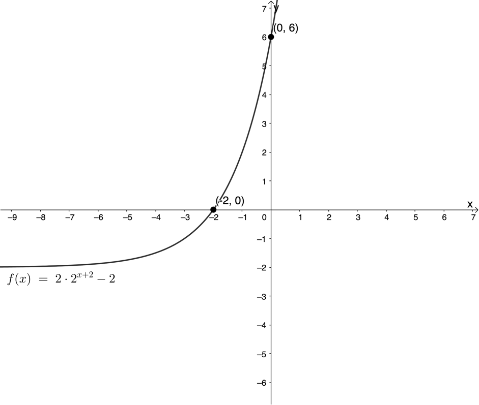
When the value of [latex]\scriptsize q[/latex] in [latex]\scriptsize y=a.{{b}^{{x+p}}}+q,b \gt 0[/latex] is zero, the graph has a horizontal asymptote that is the x-axis. In this case, the graph never crosses or even touches the x-axis and so there is no intercept with the x-axis. However, when [latex]\scriptsize q[/latex] is not equal to zero and the asymptote shifts up or down, then there may be an intercept with the x-axis. If [latex]\scriptsize a \gt 0[/latex] (and the asymptote is a minimum), the graph will intercept the x-axis if [latex]\scriptsize q \lt 0[/latex] (see Figure 4). If [latex]\scriptsize a \lt 0[/latex] (and the asymptote is a maximum), the graph will intercept the x-axis if [latex]\scriptsize q \gt 0[/latex] (see Figure 5).

To calculate the x-intercept (if it exists), we let [latex]\scriptsize x=0[/latex].

Example 5.2

Determine the intercepts with the axes of [latex]\scriptsize k(x)=2\times {{2}^{{x-4}}}-4[/latex].

Solution

Step 1: Find the y-intercept
y-intercept (let [latex]\scriptsize x=0[/latex])

[latex]\scriptsize \begin{align*}k(0) & =2\times {{2}^{{-4}}}-4\\ & =2\times \displaystyle \frac{1}{{{{2}^{4}}}}-4\\ & =2\times \displaystyle \frac{1}{{16}}-4\\ &=\displaystyle \frac{1}{8}-4\\ &=-3\displaystyle \frac{3}{8}\end{align*}[/latex]

The y-intercept is the point [latex]\scriptsize (0,-3\displaystyle \frac{3}{8})[/latex].

Step 2: Find the x-intercept (if it exists)
[latex]\scriptsize a \gt 0[/latex] and [latex]\scriptsize q \lt 0[/latex]. Therefore, we expect to find an x-intercept.

x-intercepts (let [latex]\scriptsize y=0[/latex]):
[latex]\scriptsize \begin{align*}0 & =2\times {{2}^{{x-4}}}-4\\\therefore 2\times {{2}^{{x-4}}} & =4\\\therefore {{2}^{{x-4}}} & =2\\\therefore x-4 & =1\\\therefore x & =5\end{align*}[/latex]

The x-intercept is the point [latex]\scriptsize (5,0)[/latex].

Example 5.3

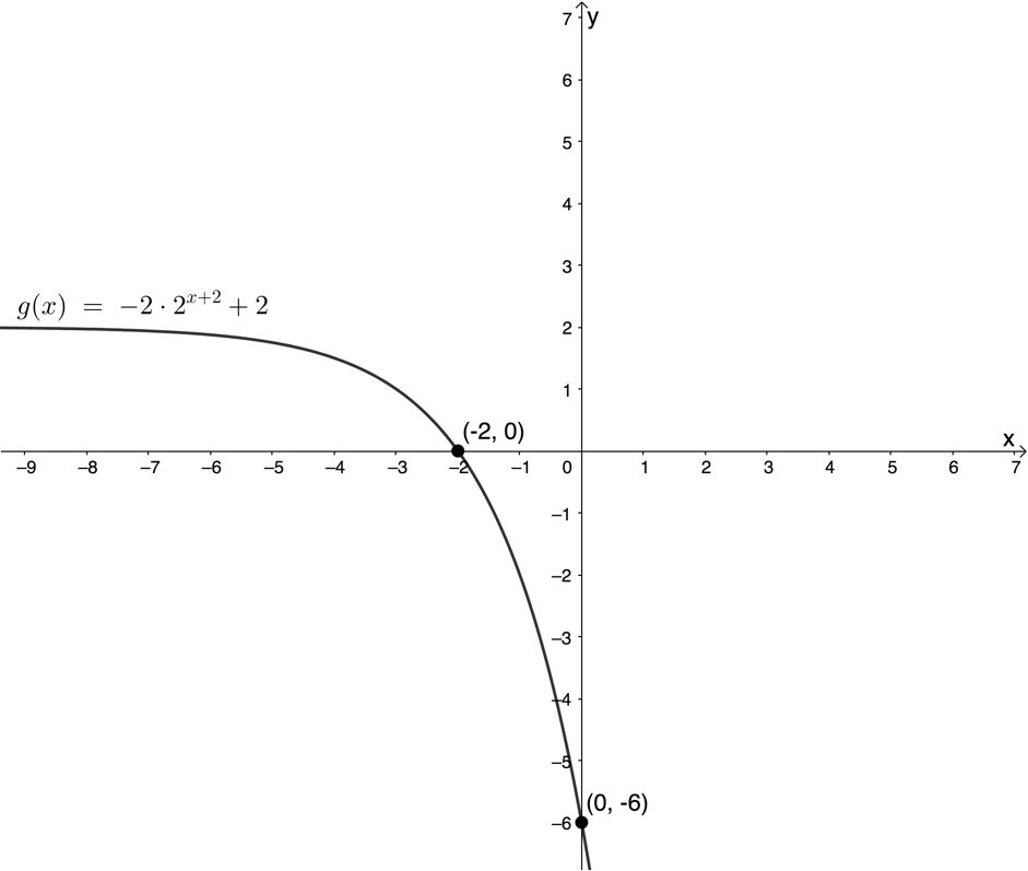
Determine the intercepts with the axes of [latex]\scriptsize m(x)=-2\times {{2}^{{x-4}}}-1[/latex].

Solution

Step 1: Find the y-intercept
y-intercept (let [latex]\scriptsize x=0[/latex])

[latex]\scriptsize \begin{align*}m(0) & =-2\times {{2}^{{-4}}}-1\\ & =-2\times \displaystyle \frac{1}{{{{2}^{4}}}}-1\\ & =-2\times \displaystyle \frac{1}{{16}}-1\\ &=-\displaystyle \frac{1}{8}-1\\ &=-1\displaystyle \frac{1}{8}\end{align*}[/latex]

The y-intercept is the point [latex]\scriptsize (0,-1\displaystyle \frac{1}{8})[/latex].

Step 2: Find the x-intercept (if it exists)
[latex]\scriptsize a \lt 0[/latex] and [latex]\scriptsize q \lt 0[/latex]. Therefore, we do not expect to find an x-intercept.

x-intercepts (let [latex]\scriptsize y=0[/latex]):
[latex]\scriptsize \begin{align*}0 & =-2\times {{2}^{{x-4}}}-1\\\therefore 2\times {{2}^{{x-4}}} & =-1\\\therefore {{2}^{{x-4}}} & =-\displaystyle \frac{1}{2}=-{{2}^{{-1}}}\end{align*}[/latex]

There are no real solutions. Therefore there is no x-intercept.

Exercise 5.2

Determine the intercepts with the axes of the following functions:

1. [latex]\scriptsize f(x)={{2}^{{x+1}}}-8[/latex]
2. [latex]\scriptsize y+18=2\times {{3}^{{x+4}}}[/latex]
3. [latex]\scriptsize \displaystyle g(x)=\left( {-\displaystyle \frac{1}{2}} \right){{\left( {\displaystyle \frac{1}{2}} \right)}^{{x-\displaystyle \frac{1}{2}}}}+4[/latex]

The full solutions are at the end of the unit.

Sketch the hyperbolic function [latex]\scriptsize y=a.{{b}^{{x+p}}}+q,b \gt 0[/latex]

Now that we are able to determine all the characteristics of the exponential function of the form [latex]\scriptsize y=a.{{b}^{{x+p}}}+q,b \gt 0[/latex], we can sketch its graph.

In order to sketch the exponential function we need to know the following:

• the basic shape
• the domain and range
• the horizontal asymptote
• the y-intercept
• the x-intercept (if it exists).

Example 5.4

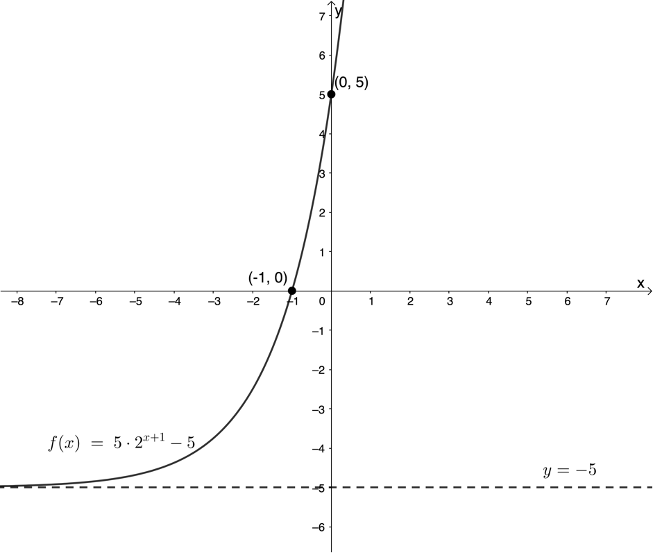
Draw a sketch of [latex]\scriptsize 2\times f(x)=10\times {{2}^{{x+1}}}-5[/latex].

Solution

First make sure that the function is in the standard form i.e. in the form [latex]\scriptsize y=a.{{b}^{{x+p}}}+q,b \gt 0[/latex].
[latex]\scriptsize \begin{align*}2\times f(x) & =10\times {{2}^{{x+1}}}-10\\\therefore f(x) & =5\times {{2}^{{x+1}}}-5\end{align*}[/latex]

Step 1: Determine the basic shape
[latex]\scriptsize a \gt 0[/latex] and [latex]\scriptsize b \gt 1[/latex] . Therefore the graph increases as [latex]\scriptsize x[/latex] increases.

Step 2: Find the domain and range
Domain: [latex]\scriptsize \{x|x\in \mathbb{R}\}\text{ }[/latex]
Range: [latex]\scriptsize a=5[/latex] therefore [latex]\scriptsize a \gt 0[/latex] so range is [latex]\scriptsize \{y|y\in \mathbb{R},y \gt q\}\text{ }[/latex]. [latex]\scriptsize q=-5[/latex] therefore the range is [latex]\scriptsize \{y|y\in \mathbb{R},y \gt -5\}\text{ }[/latex]

Step 3: Find the horizontal asymptote
From the range, we can see that the asymptote is the line [latex]\scriptsize y=-5[/latex]. The graph lies above the asymptote.

Step 4: Find the intercepts with the axes
As neither of the asymptotes is an axis, both an x- and a y-intercept exist.
y-intercept (let [latex]\scriptsize x=0[/latex]):
[latex]\scriptsize \begin{align*}f(0) & =5\times {{2}^{1}}-5\\\therefore f(0) & =5\end{align*}[/latex]
y-intercept is the point [latex]\scriptsize (0,5)[/latex]

x-intercept (let [latex]\scriptsize y=0[/latex]) ([latex]\scriptsize a \gt 0[/latex] and [latex]\scriptsize q \lt 0[/latex]) so we expect to find an x-intercept):
[latex]\scriptsize \begin{align*}0 & =5\times {{2}^{{x+1}}}-5\\\therefore 5\times {{2}^{{x+1}}} & =5\\\therefore {{2}^{{x+1}}} & =1\\\therefore x+1 & =0\\\therefore x & =-1\end{align*}[/latex]
x-intercept is the point [latex]\scriptsize (-1,0)[/latex]

Note: If the x-intercept does not exist, find one other point on the graph to help you get the right shape.

Step 5: Make a neat sketch
Draw in and label the asymptote and mark the intercepts with the axes or the other point on the graph you found. Noting the values of [latex]\scriptsize a[/latex], [latex]\scriptsize b[/latex] and the general shape of the graph, draw a smooth exponential graph passing through the points, and approaching the asymptote.

Summary

In this unit you have learnt the following:

• That the value of [latex]\scriptsize p[/latex] in [latex]\scriptsize y=a.{{b}^{{x+p}}}+q,b \gt 0[/latex] shifts the graph horizontally.
• How to determine the asymptote, domain and range of exponential functions of the form[latex]\scriptsize y=a.{{b}^{{x+p}}}+q,b \gt 0[/latex].
• How to determine the intercepts with the axes of an exponential function of the form[latex]\scriptsize y=a.{{b}^{{x+p}}}+q,b \gt 0[/latex].
• How to use the above information to make an accurate sketch of an exponential function of the form[latex]\scriptsize y=a.{{b}^{{x+p}}}+q,b \gt 0[/latex].

Unit 5: Assessment

Suggested time to complete: 30 minutes

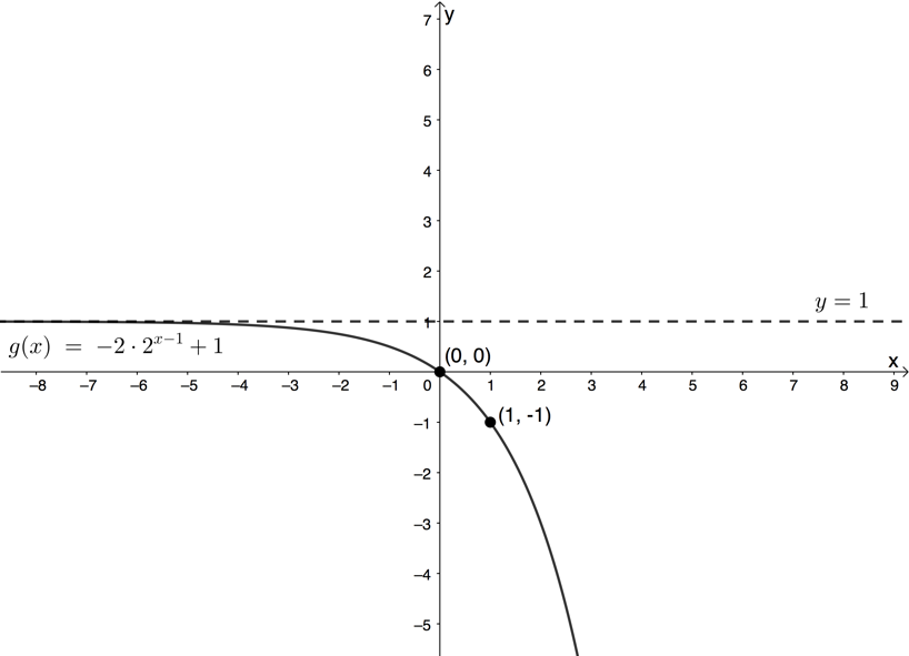
1. Given [latex]\scriptsize g(x)=-{{2.2}^{{x-1}}}+1[/latex]:
   1. What is the domain and range of [latex]\scriptsize g(x)[/latex]?
   2. Determine the asymptote of [latex]\scriptsize g(x)[/latex].
   3. For which values of [latex]\scriptsize x[/latex] is the function [latex]\scriptsize g(x)[/latex] undefined?
   4. Draw the graph of [latex]\scriptsize g(x)[/latex].
   5. Determine [latex]\scriptsize g(4)[/latex].
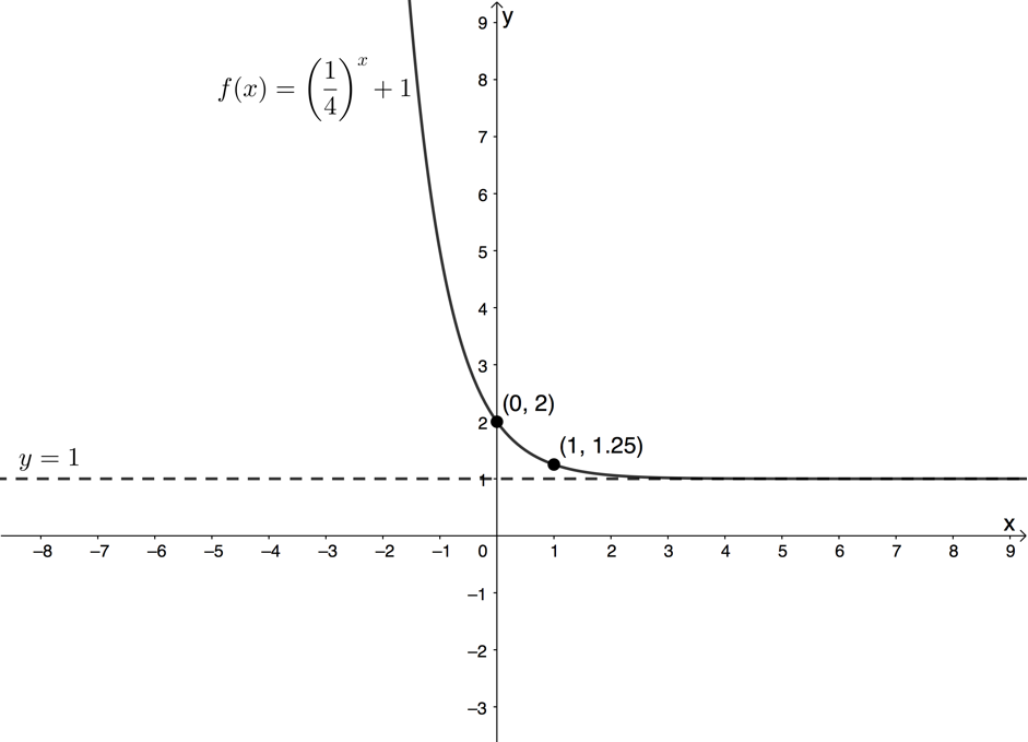
2. Given [latex]\scriptsize f(x)={{\left( {\displaystyle \frac{1}{4}} \right)}^{x}}+1[/latex]:
   1. What are the domain and range of [latex]\scriptsize f(x)[/latex]?
   2. Determine the asymptote of [latex]\scriptsize f(x)[/latex].
   3. Determine the x- and y-intercepts of [latex]\scriptsize f(x)[/latex].
   4. Draw the graph of [latex]\scriptsize f(x)[/latex].
   5. Determine [latex]\scriptsize f(-1)[/latex].

The full solutions are at the end of the unit.

Unit 5: Solutions

Exercise 5.1

1. [latex]\scriptsize y=-{{4}^{{x+3}}}-5[/latex]
   Domain: [latex]\scriptsize \{x|x\in \mathbb{R}\}\text{ }[/latex]
   Range: [latex]\scriptsize a=-1[/latex] therefore [latex]\scriptsize a \lt 0[/latex] so range is [latex]\scriptsize \{y|y\in \mathbb{R},y \lt q\}\text{ }[/latex]. [latex]\scriptsize q=-5[/latex] therefore range is [latex]\scriptsize \{y|y\in \mathbb{R},y \lt -5\}\text{ }[/latex]
   Horizontal asymptote is the line [latex]\scriptsize y=-5[/latex]
2. [latex]\scriptsize \begin{align*}y+3 & ={{3}^{{x-3}}}\\\therefore y & ={{3}^{{x-3}}}-3\end{align*}[/latex]
   Domain: [latex]\scriptsize \{x|x\in \mathbb{R}\}\text{ }[/latex]
   Range: [latex]\scriptsize a=1[/latex] therefore [latex]\scriptsize a \gt 0[/latex] so range is [latex]\scriptsize \{y|y\in \mathbb{R},y \gt q\}\text{ }[/latex]. [latex]\scriptsize q=-3[/latex] therefore range is [latex]\scriptsize \{y|y\in \mathbb{R},y \gt -3\}\text{ }[/latex]
   Horizontal asymptote is the line [latex]\scriptsize y=-3[/latex]
3. [latex]\scriptsize \begin{align*}\displaystyle \frac{y}{{-2}} & ={{3}^{{x+1}}}-1\\\therefore y & =-2\times {{3}^{{x+1}}}+2\end{align*}[/latex]
   Domain: [latex]\scriptsize \{x|x\in \mathbb{R}\}\text{ }[/latex]
   Range: [latex]\scriptsize a=-2[/latex] therefore [latex]\scriptsize a \lt 0[/latex] so range is [latex]\scriptsize \{y|y\in \mathbb{R},y \lt q\}\text{ }[/latex]. [latex]\scriptsize q=2[/latex] therefore range is [latex]\scriptsize \{y|y\in \mathbb{R},y \lt 2\}\text{ }[/latex]
   Horizontal asymptote is the line [latex]\scriptsize y=2[/latex]
4. [latex]\scriptsize f(x)={{\left( {\displaystyle \frac{1}{2}} \right)}^{{x+3}}}[/latex]
   Domain: [latex]\scriptsize \{x|x\in \mathbb{R}\}\text{ }[/latex]
   Range: [latex]\scriptsize a=1[/latex] therefore [latex]\scriptsize a \gt 0[/latex] so range is [latex]\scriptsize \{y|y\in \mathbb{R},y \gt q\}\text{ }[/latex]. [latex]\scriptsize q=0[/latex] therefore range is [latex]\scriptsize \{y|y\in \mathbb{R},y \gt 0\}\text{ }[/latex]
   Horizontal asymptote is the line [latex]\scriptsize y=0[/latex]

Back to Exercise 5.1

Exercise 5.2

1. .
   y-intercept (let [latex]\scriptsize x=0[/latex])
   [latex]\scriptsize \begin{align*}f(0)&={{2}^{1}}-8\\&=-6\end{align*}[/latex]
   y-intercept is the point [latex]\scriptsize (0,-6)[/latex].
   x-intercept (let [latex]\scriptsize y=0[/latex]) ([latex]\scriptsize a \gt 0[/latex], [latex]\scriptsize q \lt 0[/latex] so we expect to find an x-intercept)
   [latex]\scriptsize \begin{align*}0 & ={{2}^{{x+1}}}-8\\\therefore {{2}^{{x+1}}} & =8={{2}^{3}}\\\therefore x+1 & =3\\\therefore x & =2\end{align*}[/latex]
   x-intercept is the point [latex]\scriptsize (2,0)[/latex].
2. .
   [latex]\scriptsize \begin{align*}y+18 & =2\times {{3}^{{x+4}}}\\\therefore y & =2\times {{3}^{{x+4}}}-18\end{align*}[/latex]
   y-intercept (let [latex]\scriptsize x=0[/latex])
   [latex]\scriptsize \begin{align*}y&=2\times {{3}^{4}}-18\\&=2\times 81-18\\&=144\end{align*}[/latex]
   y-intercept is the point [latex]\scriptsize (0,144)[/latex].
   x-intercept (let [latex]\scriptsize y=0[/latex]) ([latex]\scriptsize a \gt 0[/latex], [latex]\scriptsize q \lt 0[/latex] so we expect to find an x-intercept)
   [latex]\scriptsize \begin{align*}0 & =2\times {{3}^{{x+4}}}-18\\\therefore 2\times {{3}^{{x+4}}} & =18\\\therefore {{3}^{{x+4}}} & =9={{3}^{2}}\\\therefore x+4 & =2\\\therefore x & =-2\end{align*}[/latex]
   x-intercept is the point [latex]\scriptsize (-2,0)[/latex].
3. .
   y-intercept (let [latex]\scriptsize x=0[/latex])
   [latex]\scriptsize \begin{align*}g(0)&=\left( {-\displaystyle \frac{1}{2}} \right){{\left( {\displaystyle \frac{1}{2}} \right)}^{{-\displaystyle \frac{1}{2}}}}+4\\&=-\displaystyle \frac{1}{2}\times \displaystyle \frac{1}{{{{{\left( {\displaystyle \frac{1}{2}} \right)}}^{{\frac{1}{2}}}}}}+4\\&=-\displaystyle \frac{1}{2}\times \displaystyle \frac{1}{{\sqrt{{\displaystyle \frac{1}{2}}}}}+4\\&=-\displaystyle \frac{1}{{\left( {\displaystyle \frac{2}{{\sqrt{2}}}} \right)}}+4\\&=-\displaystyle \frac{{\sqrt{2}}}{2}+4\end{align*}[/latex]
   y-intercept is the point [latex]\scriptsize (0,-\displaystyle \frac{{\sqrt{2}}}{2}+4)[/latex].
   x-intercept (let [latex]\scriptsize y=0[/latex]) ([latex]\scriptsize a \lt 0[/latex], [latex]\scriptsize q \gt 0[/latex] so we expect to find an x-intercept)
   [latex]\scriptsize \begin{align*}0 & =\left( {-\displaystyle \frac{1}{2}} \right){{\left( {\displaystyle \frac{1}{2}} \right)}^{{x-\displaystyle \frac{1}{2}}}}+4\\\therefore \left( {\displaystyle \frac{1}{2}} \right){{\left( {\displaystyle \frac{1}{2}} \right)}^{{x-\displaystyle \frac{1}{2}}}} & =4\\\therefore {{\left( {\displaystyle \frac{1}{2}} \right)}^{{x-\displaystyle \frac{1}{2}}}} & =8={{2}^{3}}\\\therefore {{2}^{{-\left( {x-\displaystyle \frac{1}{2}} \right)}}} & ={{2}^{3}}\\\therefore -x+\displaystyle \frac{1}{2} & =3\\\therefore x & =-\displaystyle \frac{5}{2}\end{align*}[/latex]
   x-intercept is the point [latex]\scriptsize (-\displaystyle \frac{5}{2},0)[/latex].

Back to Exercise 5.2

Unit 5: Assessment

1. [latex]\scriptsize g(x)=-{{2.2}^{{x-1}}}+1[/latex]
   1. Domain: [latex]\scriptsize \{x|x\in \mathbb{R}\}\text{ }[/latex]
      Range: [latex]\scriptsize a=-2[/latex] therefore [latex]\scriptsize a \lt 0[/latex] so range is [latex]\scriptsize \{y|y\in \mathbb{R},y \lt q\}\text{ }[/latex]. [latex]\scriptsize q=1[/latex] therefore range is [latex]\scriptsize \{y|y\in \mathbb{R},y \lt 1\}\text{ }[/latex]
   2. [latex]\scriptsize y=1[/latex]
   3. The function is not undefined for any values of [latex]\scriptsize x[/latex].
   4. [latex]\scriptsize a \lt 0[/latex] and [latex]\scriptsize b \gt 1[/latex]. Therefore, the graph decreases as [latex]\scriptsize x[/latex] increases.
      Before we can draw the graph, we need to find the intercepts on the axes.
      y-intercept (let [latex]\scriptsize x=0[/latex])
      [latex]\scriptsize \begin{align*}g(0)&=-{{2.2}^{{-1}}}+1\\&=-2.\displaystyle \frac{1}{2}+1\\&=0\end{align*}[/latex]
      y-intercept is the point [latex]\scriptsize (0,0)[/latex].
      The graph passes through the origin. Therefore, we need to find one other point on the graph to help get the right shape.
      [latex]\scriptsize \begin{align*}g(1)&=-{{2.2}^{{1-1}}}+1\\&=-{{2.2}^{0}}+1\\&=-2+1\\&=-1\end{align*}[/latex]
      The point [latex]\scriptsize (1,-1)[/latex] lies on the graph.
      
   5. .
      [latex]\scriptsize \begin{align*} g(4)&=-2\cdot 2^{x-1}+1\\ &=-2\cdot 2^3+1\\ &=-16^1\\ &=-15 \end{align*}[/latex]
2. [latex]\scriptsize f(x)={{\left( {\displaystyle \frac{1}{4}} \right)}^{x}}+1[/latex]
   1. Domain: [latex]\scriptsize \{x|x\in \mathbb{R}\}\text{ }[/latex]
      Range: [latex]\scriptsize a=1[/latex] therefore [latex]\scriptsize a \gt 0[/latex] so range is [latex]\scriptsize \{y|y\in \mathbb{R},y \gt q\}\text{ }[/latex]. [latex]\scriptsize q=1[/latex] therefore range is [latex]\scriptsize \{y|y\in \mathbb{R},y \gt 1\}\text{ }[/latex]
   2. [latex]\scriptsize y=1[/latex]
   3. y-intercept (let [latex]\scriptsize x=0[/latex])
      [latex]\scriptsize \begin{align*}f(0)&={{\left( {\displaystyle \frac{1}{4}} \right)}^{0}}+1\\&=1+1\\&=2\end{align*}[/latex]
      y-intercept is the point [latex]\scriptsize (0,2)[/latex].
      x-intercept (let [latex]\scriptsize y=0[/latex])
      [latex]\scriptsize a \gt 0[/latex] and [latex]\scriptsize q \gt 1[/latex]. Therefore, there is no x-intercept. We choose another x-value to find another point on the graph to help with the drawing. Let [latex]\scriptsize x=1[/latex].
      [latex]\scriptsize \begin{align*}f(1)&={{\left( {\displaystyle \frac{1}{4}} \right)}^{1}}+1\\&=\displaystyle \frac{5}{4}\end{align*}[/latex]
      The point [latex]\scriptsize (1,\displaystyle \frac{5}{4})[/latex] lies on the graph.
   4. [latex]\scriptsize a \gt 0[/latex] and [latex]\scriptsize 0 \lt b \lt 1[/latex]. Therefore, the graph increases as [latex]\scriptsize x[/latex] decreases.
      
   5. .
      [latex]\scriptsize \begin{align*}f(-1)&={{\left( {\displaystyle \frac{1}{4}} \right)}^{{-1}}}+1\\&=4+1\\&=5\end{align*}[/latex]

Back to Unit 5: Assessment