Functions and algebra: Use a variety of techniques to sketch and interpret information from graphs of functions
Unit 11: The tangent function
Dylan Busa
Unit outcomes
By the end of this unit you will be able to:
- Sketch functions of the form [latex]\scriptsize y=a\tan k\theta[/latex].
- Determine the effects of [latex]\scriptsize a[/latex] and [latex]\scriptsize k[/latex] on the tangent graph of the form [latex]\scriptsize y=a\tan k\theta[/latex].
- Find the values of [latex]\scriptsize a[/latex] and [latex]\scriptsize k[/latex] from a given tangent graph of the form [latex]\scriptsize y=a\tan k\theta[/latex].
Remember that the domain of trigonometric functions can be represented as [latex]\scriptsize x[/latex] or [latex]\scriptsize \theta[/latex]. Therefore, [latex]\scriptsize y=\tan x[/latex] and [latex]\scriptsize y=\tan \theta[/latex] are the same function.
What you should know
Before you start this unit, make sure you can:
- Sketch tangent functions of the form [latex]\scriptsize y=a\tan \theta +q[/latex]. Refer to level 2 subject outcome 2.1 Unit 5 if you need help with this.
Introduction
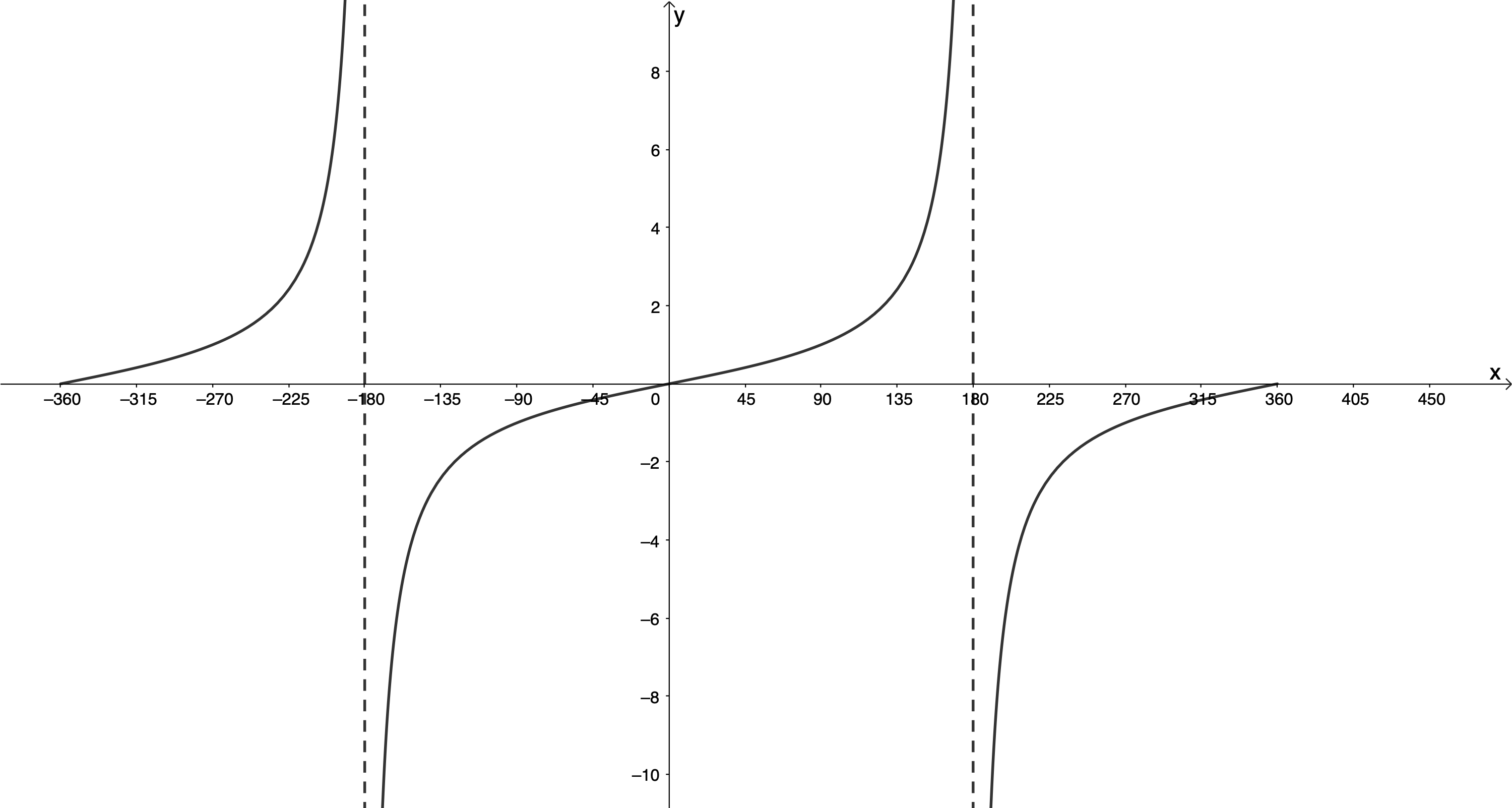
We know that the period of the tangent function [latex]\scriptsize y=\tan \theta[/latex] is [latex]\scriptsize {{180}^\circ}[/latex] (see Figure 1). The period of the tangent function is different from the sine and cosine functions and, as we can see in Figure 1, the shape of the function is also different. Instead of having regular repeated maximum and minimum turning points, the tangent function increases to positive and negative infinity on either side of vertical asymptotes. Remember that the function [latex]\scriptsize y=\tan x[/latex] is undefined for the values of [latex]\scriptsize x[/latex]at these asymptotes.
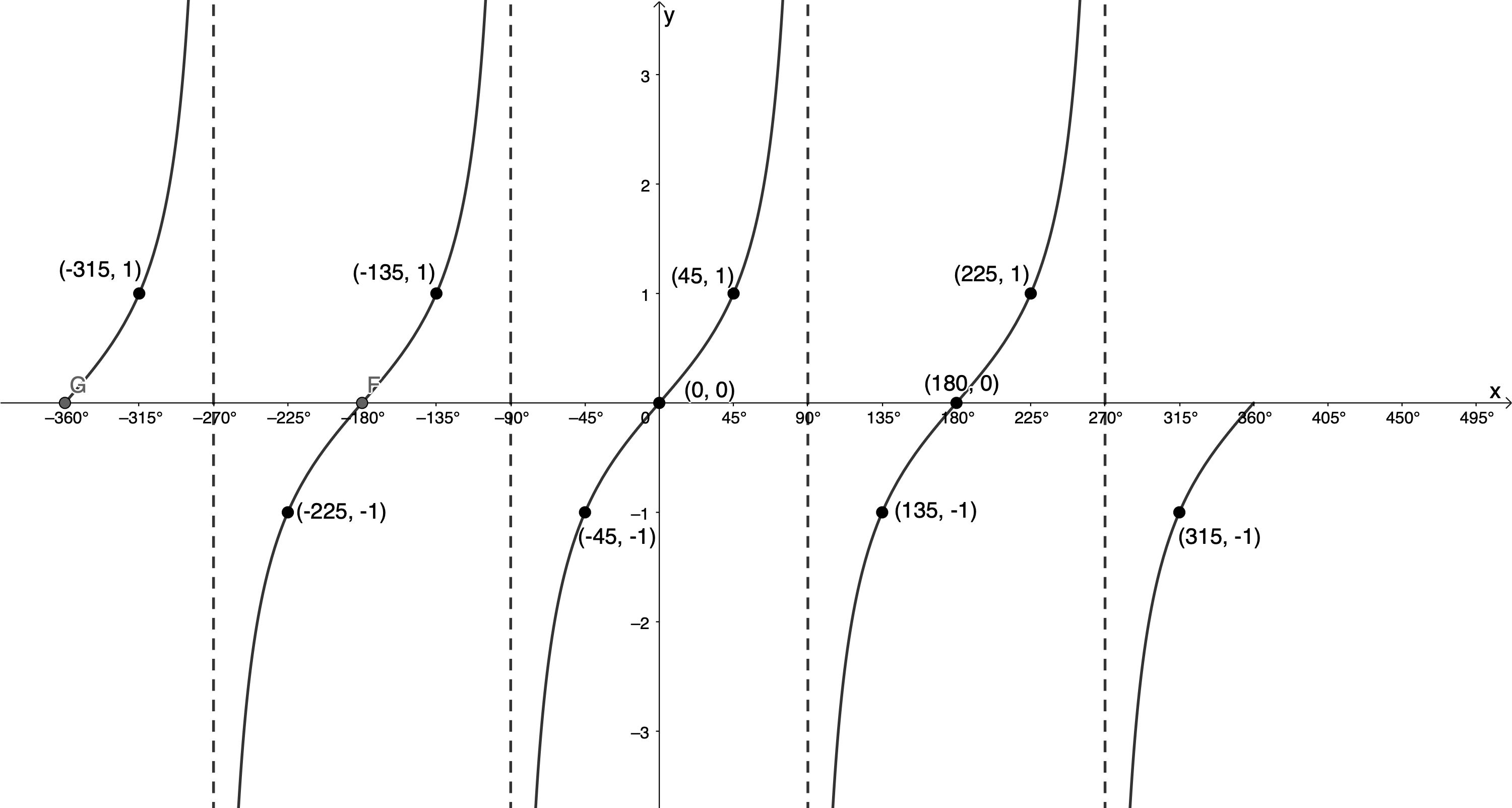
Because the tangent function does not have maximum and minimum turning points and increases to positive and negative infinity, we cannot say that it has an amplitude. However, the function [latex]\scriptsize y=\tan x[/latex] does pass through the points [latex]\scriptsize ({{45}^\circ},1)[/latex] and [latex]\scriptsize ({{225}^\circ},1)[/latex] and [latex]\scriptsize ({{135}^\circ},-1)[/latex] and [latex]\scriptsize ({{225}^\circ},-1)[/latex] in the interval [latex]\scriptsize {{0}^\circ}\le x\le {{360}^\circ}[/latex] (see Figure 1) which are important ‘anchor points’ when it comes to sketching the tangent function.
In level 2 we were introduced to the tangent function of the form [latex]\scriptsize y=a\tan \theta +q[/latex]. We discovered that the value of [latex]\scriptsize q[/latex] shifted the graph vertically up and down while the value of [latex]\scriptsize a[/latex] changed the shape of the graph.
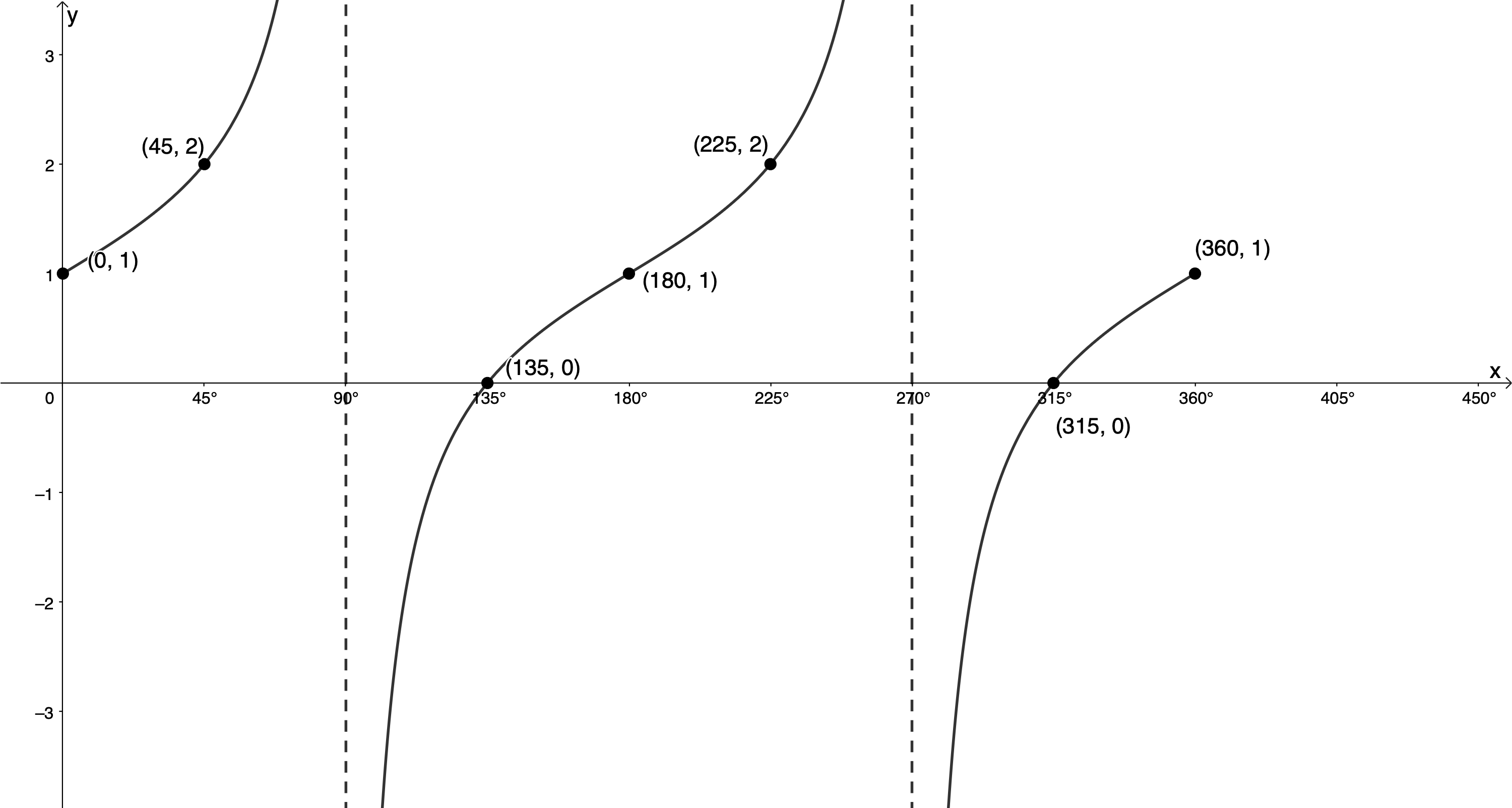
For example, for the function [latex]\scriptsize y=\tan x+1[/latex], each of these ‘anchor points’ is shifted [latex]\scriptsize 1[/latex] unit up (see Figure 2). The point [latex]\scriptsize ({{0}^\circ},0)[/latex] becomes the point [latex]\scriptsize ({{0}^\circ},1)[/latex], the point [latex]\scriptsize ({{45}^\circ},1)[/latex] becomes the point [latex]\scriptsize ({{45}^\circ},2)[/latex], the point [latex]\scriptsize ({{135}^\circ},-1)[/latex] becomes the point [latex]\scriptsize ({{135}^\circ},0)[/latex] and so on.
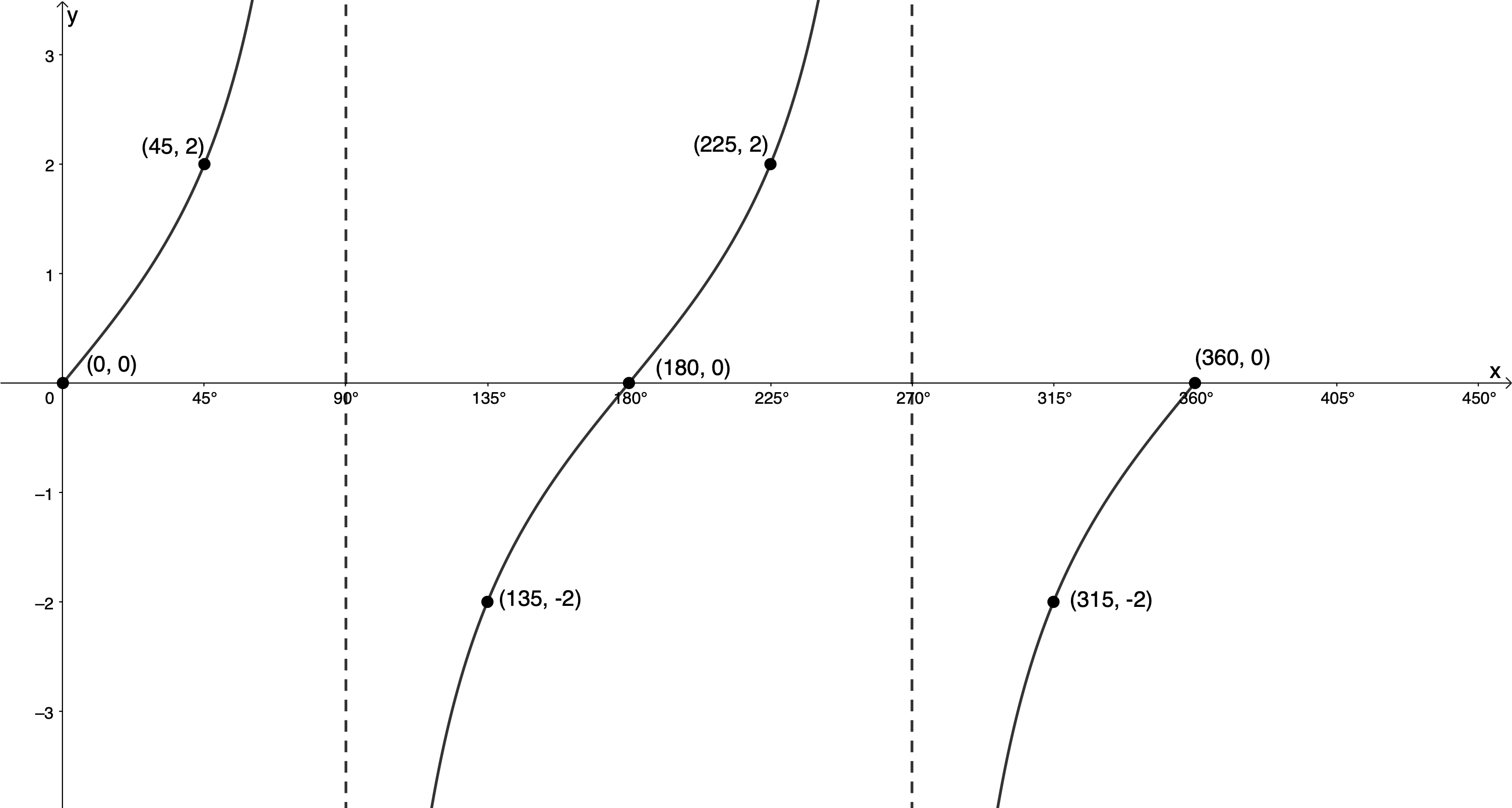
And for the function [latex]\scriptsize y=2\tan x[/latex], each of these ‘anchor points’ have y-values of [latex]\scriptsize 2[/latex] or [latex]\scriptsize -2[/latex] respectively (see Figure 3).
Take note!
Period of [latex]\scriptsize y=a\tan \theta +q[/latex] is [latex]\scriptsize {{180}^\circ}[/latex].
The effect of [latex]\scriptsize q[/latex]:
- if [latex]\scriptsize q \gt 0[/latex], the function is shifted up by [latex]\scriptsize q[/latex] units
- if [latex]\scriptsize q \lt 0[/latex], the function is shifted down by [latex]\scriptsize q[/latex] units.
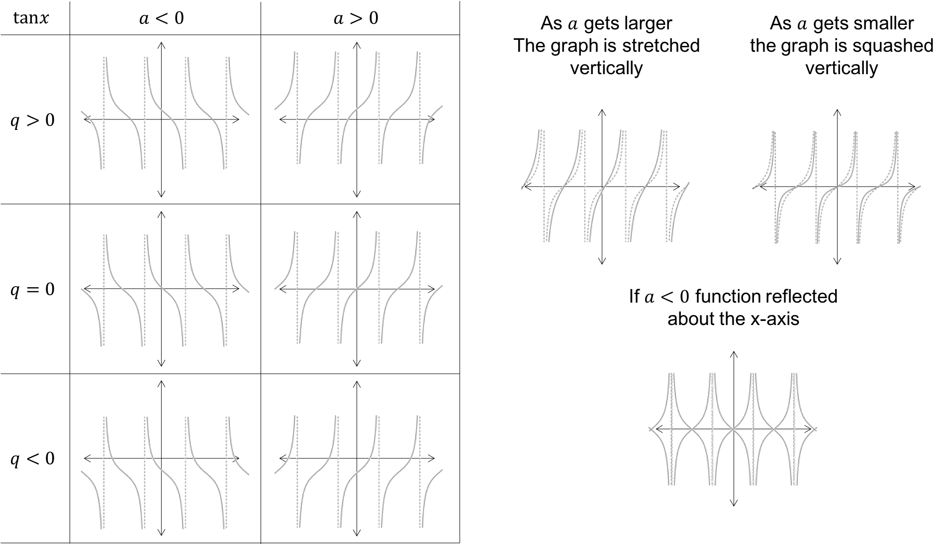
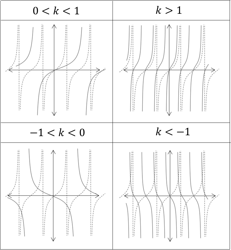
The effect of [latex]\scriptsize a[/latex]:
- if [latex]\scriptsize a \gt 1[/latex], the branches of the function are steeper
- if [latex]\scriptsize 0 \lt a \lt 1[/latex], the branches of the function are less steep (the function bends more)
- if [latex]\scriptsize a \lt 0[/latex], the function is reflected about the x-axis
- if [latex]\scriptsize -1 \lt a \lt 0[/latex], the function is reflected about the x-axis and the branches of the function are less steep (the function bends more)
- if [latex]\scriptsize a \lt -1[/latex], the function is reflected about the x-axis and the branches of the function are steeper.
Note
If you have access to the internet, visit this interactive simulation.
Here you will find a tangent function of the form [latex]\scriptsize y=a\tan x+q[/latex] with sliders to change the values of [latex]\scriptsize a[/latex] and [latex]\scriptsize q[/latex]. Spend some time playing with it to make sure that you understand how changing the values of [latex]\scriptsize a[/latex] and [latex]\scriptsize q[/latex] affects the shape and location of the tangent function of the form [latex]\scriptsize y=a\tan x+q[/latex].
The tangent function of the form [latex]\scriptsize y=\tan kx[/latex]
In Activity 7.1 in unit 7, we saw that the value of [latex]\scriptsize k[/latex] in [latex]\scriptsize y=\sin kx[/latex] affects the period of the function and that we can calculate the period as [latex]\scriptsize \text{period}=\displaystyle \frac{{{{{360}}^\circ}}}{{\left| k \right|}}[/latex] where [latex]\scriptsize \left| k \right|\text{ }[/latex] is the absolute value of [latex]\scriptsize k[/latex], in other words the positive value of [latex]\scriptsize k[/latex].
This means that if [latex]\scriptsize k \gt 1[/latex], the period decreases and if [latex]\scriptsize 0 \lt k \lt 1[/latex], the period increases.
The same is true for the tangent function [latex]\scriptsize y=\tan kx[/latex]. Remember that the period of [latex]\scriptsize y=\tan x[/latex] is [latex]\scriptsize {{180}^\circ}[/latex]. Therefore, the period can be calculated as follows:
[latex]\scriptsize \text{Period}=\displaystyle \frac{{{{{180}}^\circ}}}{{\left| k \right|}}\text{ }[/latex] where [latex]\scriptsize \left| k \right|\text{ }[/latex] is the absolute value of [latex]\scriptsize k[/latex], in other words the positive value of [latex]\scriptsize k[/latex].
This means that if [latex]\scriptsize k \gt 1[/latex], the period decreases and if [latex]\scriptsize 0 \lt k \lt 1[/latex], the period increases.
If [latex]\scriptsize k \lt 0[/latex], it changes the period AND reflects the graph about the x-axis because [latex]\scriptsize \tan (-x)=-\tan (x)[/latex].
Note
If you have an internet connection, visit this online simulation to compare the effects values of [latex]\scriptsize k \lt 0[/latex] have on the sine, cosine and tangent functions.
Take note!
In [latex]\scriptsize y=\tan kx[/latex] the [latex]\scriptsize \text{Period}=\displaystyle \frac{{{{{180}}^\circ}}}{{\left| k \right|}}\text{ }[/latex].
[latex]\scriptsize \tan (-x)=-\tan (x)[/latex]. Therefore, if [latex]\scriptsize k \lt 0[/latex], it changes the period AND reflects the graph about the x-axis.
Example 11.1
Given the function [latex]\scriptsize y=\tan \left( {\displaystyle \frac{{2x}}{3}} \right)[/latex] for the interval [latex]\scriptsize {{0}^\circ}\le x\le {{360}^\circ}[/latex], determine the:
- period
- location of the vertical asymptotes
- domain and range.
Solutions
- [latex]\scriptsize k=\displaystyle \frac{2}{3}[/latex]. Therefore, the period of the graph is [latex]\scriptsize \displaystyle \frac{{{{{180}}^\circ}}}{{\left| {\displaystyle \frac{2}{3}} \right|}}=\displaystyle \frac{{3\times {{{180}}^\circ}}}{2}={{270}^\circ}[/latex].
- The new period is [latex]\scriptsize {{270}^\circ}[/latex]. This means that the asymptotes have also changed. There used to be an asymptote at [latex]\scriptsize {{90}^\circ}[/latex], in the middle of the original period of [latex]\scriptsize {{180}^\circ}[/latex]. The new asymptote will still be in the middle of the period. There are two ways to calculate the value of this new asymptote.[latex]\scriptsize \text{new asymptote}=\displaystyle \frac{{\text{period}}}{{2}}=\displaystyle \frac{{{{{270}}^\circ}}}{{2}}={{135}^\circ}[/latex], or
[latex]\scriptsize \text{new asymptote}=\displaystyle \frac{{\text{original asymptote}}}{{\left| k \right|}}=\displaystyle \frac{{{{{90}}^\circ}}}{{\displaystyle \frac{2}{3}}}=\displaystyle \frac{{3\times {{{90}}^\circ}}}{2}={{135}^\circ}[/latex]In [latex]\scriptsize y=\tan x[/latex] we also know that the vertical asymptotes are [latex]\scriptsize {{180}^\circ}[/latex] or one period apart. The new asymptotes will also be one period apart. Therefore, the next asymptote to the right will be at [latex]\scriptsize {{135}^\circ}+{{270}^\circ}={{405}^\circ}[/latex] which is outside of the given interval. The next asymptote to the left will be [latex]\scriptsize {{135}^\circ}-{{270}^\circ}=-{{135}^\circ}[/latex] which is also outside the given interval. Therefore, the only asymptote within our interval is [latex]\scriptsize x={{135}^\circ}[/latex].
- Domain: [latex]\scriptsize \{x|x\in \mathbb{R},{{0}^\circ}\le x\le {{360}^\circ},x\ne {{135}^\circ}\}\text{ }[/latex]
Range: [latex]\scriptsize \{y|y\in \mathbb{R}\}\text{ }[/latex]
Remember that the tangent function does not have maximum and minimum turning points. Therefore, the range is all real values.
Exercise 11.1
- Determine the periods and the location of the asymptotes for the following functions:
- [latex]\scriptsize y=\tan (2x)[/latex]
- [latex]\scriptsize y=\tan \left( {-\displaystyle \frac{3}{5}x} \right)[/latex]
- [latex]\scriptsize \displaystyle y=\tan \left( {-\displaystyle \frac{3}{2}x} \right)[/latex]
- For each function of the form [latex]\scriptsize y=\tan kx[/latex], determine the value of [latex]\scriptsize k[/latex]:
- .
- .
- .
- .
The full solutions are at the end of the unit.
Sketch functions of the form [latex]\scriptsize y=a\tan kx[/latex]
Now that we know that the value of [latex]\scriptsize k[/latex] affects the period of the function [latex]\scriptsize y=\tan kx[/latex], we can combine this with our knowledge of the effects of [latex]\scriptsize a[/latex], and examine functions of the form [latex]\scriptsize y=a\tan kx[/latex].
The effects of [latex]\scriptsize a[/latex] on [latex]\scriptsize y=a\tan kx[/latex] are exactly the same as they were on [latex]\scriptsize y=a\tan x+q[/latex]. Before we learn how to sketch functions of the form [latex]\scriptsize y=a\tan kx[/latex], spend some time playing with this online simulation.
Here you will find a graph of the function [latex]\scriptsize y=a\tan kx+q[/latex] for the interval [latex]\scriptsize -{{360}^\circ}\le x\le {{360}^\circ}[/latex]. Pay particular attention to how the position of the asymptotes, the value of the ‘anchor points’ (including the intercepts with the x-axis), the shape of the branches of the graph and the period change as you change the values of [latex]\scriptsize a[/latex], [latex]\scriptsize k[/latex] and [latex]\scriptsize q[/latex].
The best way to sketch functions of the form [latex]\scriptsize y=a\tan kx[/latex] is to transform the basic function of [latex]\scriptsize y=\tan x[/latex] depending on the values of [latex]\scriptsize a[/latex] and [latex]\scriptsize k[/latex]. To do this, you need to know the set of ‘anchor points’ of [latex]\scriptsize y=\tan x[/latex], as transformation of these points will help you to sketch functions of the form [latex]\scriptsize y=a\tan kx[/latex].
Take note!
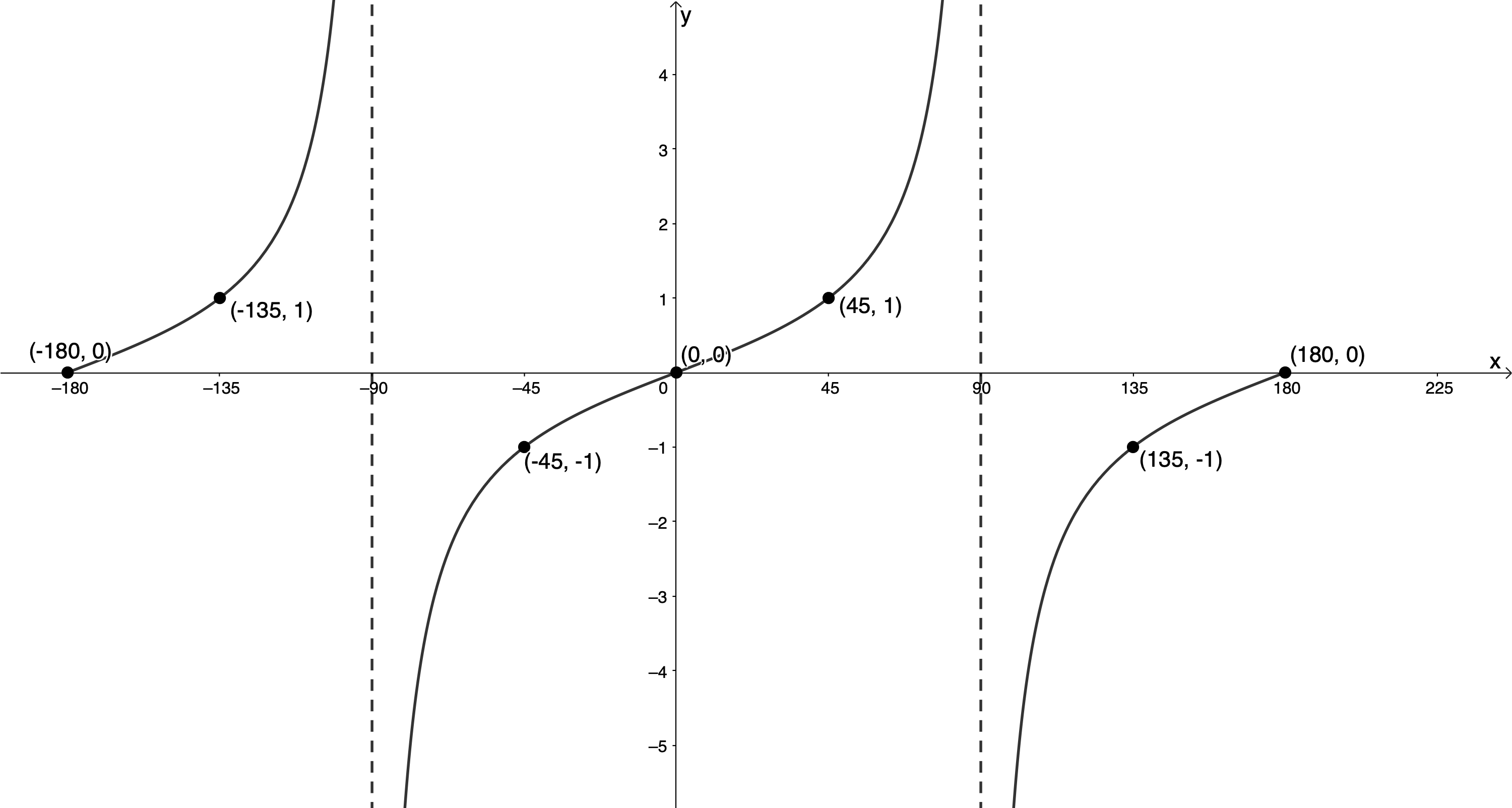
The ‘anchor points’ for [latex]\scriptsize y=\tan x[/latex] are illustrated in Figure 5 for the interval [latex]\scriptsize -{{180}^\circ}\le x\le {{180}^\circ}[/latex].
Example 11.2
Sketch the function [latex]\scriptsize y=2\tan 2x[/latex] for the interval [latex]\scriptsize -{{90}^\circ}\le x\le {{90}^\circ}[/latex].
Solution
The function is of the form [latex]\scriptsize y=a\tan kx[/latex]. Therefore, [latex]\scriptsize a=2[/latex] and [latex]\scriptsize k=2[/latex]. Because [latex]\scriptsize k=2[/latex], we know that the period of the function will be [latex]\scriptsize \displaystyle \frac{{{{{180}}^\circ}}}{{\left| 2 \right|}}={{90}^\circ}[/latex]. We need to transform one period of ‘anchor points’ as follows:
| [latex]\scriptsize \tan x[/latex] | [latex]\scriptsize ({{0}^\circ},0)[/latex] | [latex]\scriptsize ({{45}^\circ},1)[/latex] | [latex]\scriptsize x={{90}^\circ}[/latex] asymptote | [latex]\scriptsize ({{135}^\circ},-1)[/latex] | [latex]\scriptsize ({{180}^\circ},0)[/latex] |
| [latex]\scriptsize \tan 2x[/latex] | [latex]\scriptsize ({{0}^\circ},0)[/latex] | [latex]\scriptsize ({{22.5}^\circ},1)[/latex] | [latex]\scriptsize x={{45}^\circ}[/latex] asymptote |
[latex]\scriptsize ({{67.5}^\circ},-1)[/latex] | [latex]\scriptsize ({{90}^\circ},0)[/latex] |
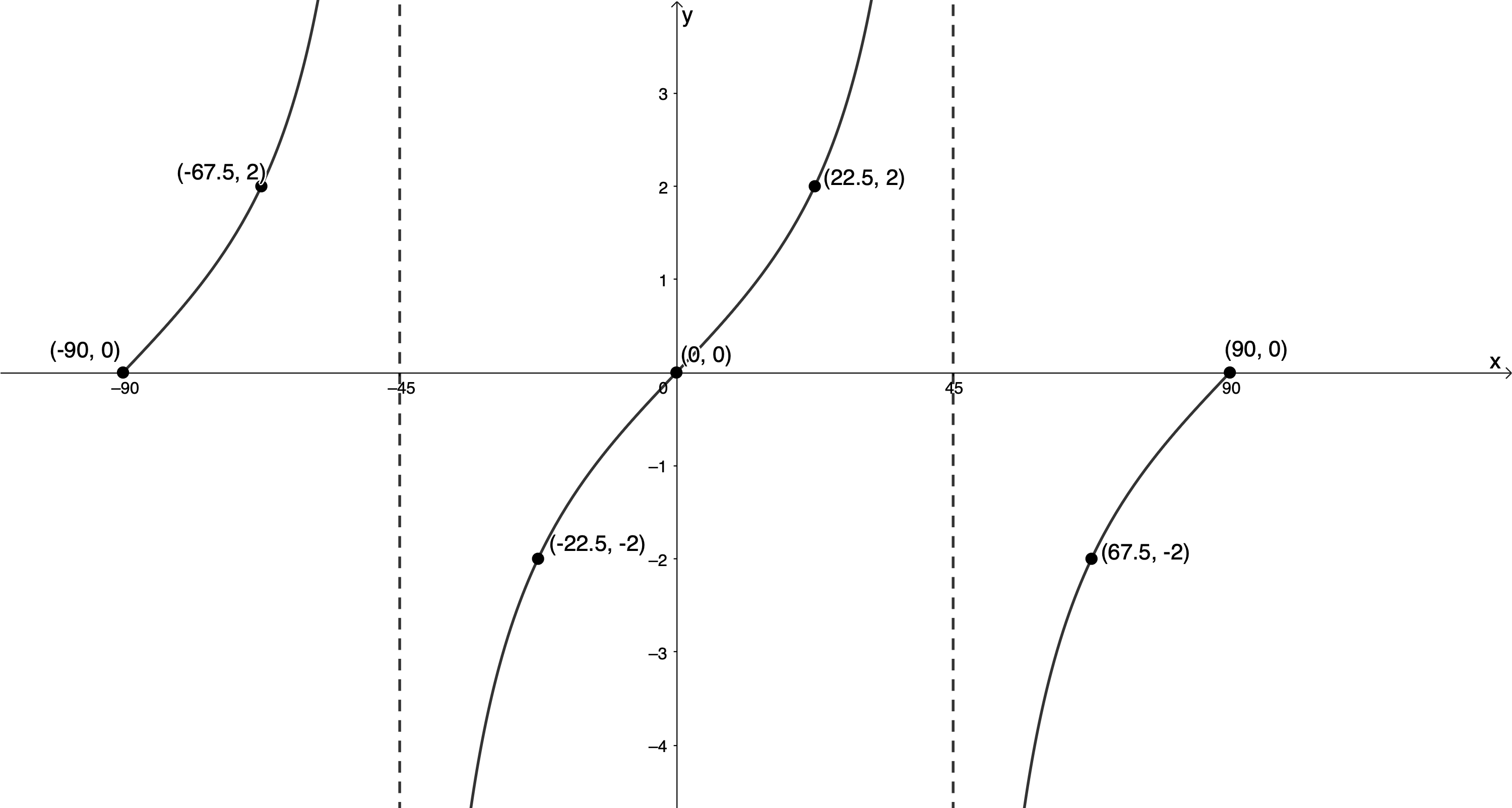
Because the period has been halved, the value of each of the x-coordinates is also halved. We can see that the function will start at [latex]\scriptsize 0[/latex], pass through [latex]\scriptsize ({{22.5}^\circ},1)[/latex] as it increases to infinity approaching the asymptote from the left , decrease to negative infinity as it approaches the asymptote from the right, pass through the point [latex]\scriptsize ({{67.5}^\circ},-1)[/latex], rise back to zero at [latex]\scriptsize {{90}^\circ}[/latex], the new period.
Because [latex]\scriptsize a=2[/latex], we know that each function value (or y-value) is going to be multiplied by [latex]\scriptsize 2[/latex] thereby stretching the branches of the function out by a factor of [latex]\scriptsize 2[/latex]. We need to further transform one period of ‘anchor points’ as follows:
| [latex]\scriptsize \tan x[/latex] | [latex]\scriptsize ({{0}^\circ},0)[/latex] | [latex]\scriptsize ({{45}^\circ},1)[/latex] | [latex]\scriptsize x={{90}^\circ}[/latex] asymptote | [latex]\scriptsize ({{135}^\circ},-1)[/latex] | [latex]\scriptsize ({{180}^\circ},0)[/latex] |
| [latex]\scriptsize \tan 2x[/latex] | [latex]\scriptsize ({{0}^\circ},0)[/latex] | [latex]\scriptsize ({{22.5}^\circ},1)[/latex] | [latex]\scriptsize x={{45}^\circ}[/latex] asymptote | [latex]\scriptsize ({{67.5}^\circ},-1)[/latex] | [latex]\scriptsize ({{90}^\circ},0)[/latex] |
[latex]\scriptsize 2\tan 2x[/latex] [latex]\scriptsize ({{0}^\circ},0)[/latex] [latex]\scriptsize ({{22.5}^\circ},2)[/latex] [latex]\scriptsize x={{45}^\circ}[/latex] asymptote [latex]\scriptsize ({{67.5}^\circ},-2)[/latex] [latex]\scriptsize ({{90}^\circ},0)[/latex]
We can see that the function will start at [latex]\scriptsize 0[/latex], pass through [latex]\scriptsize ({{22.5}^\circ},2)[/latex] as it increases to infinity approaching the asymptote from the left , decrease to negative infinity as it approaches the asymptote from the right, pass through the point [latex]\scriptsize ({{67.5}^\circ},-2)[/latex], rise back to zero at [latex]\scriptsize {{90}^\circ}[/latex], the new period.
We can now plot our transformed ‘anchor points’ and draw the graph. We first draw it for the interval [latex]\scriptsize {{0}^\circ}\le x\le {{90}^\circ}[/latex] and then continue to pattern for the full interval of [latex]\scriptsize -{{90}^\circ}\le x\le {{90}^\circ}[/latex].
Example 11.3
Given the function [latex]\scriptsize f(x)=3\tan \left( {-\displaystyle \frac{1}{2}x} \right)[/latex].
- Sketch the graph of [latex]\scriptsize f(x)[/latex] for the interval [latex]\scriptsize -{{180}^\circ}\le x\le {{180}^\circ}[/latex].
- State the asymptotes within the interval.
- State the domain and range of [latex]\scriptsize f(x)[/latex].
- What is the period of [latex]\scriptsize f(x)[/latex]?
Solutions
- The function is of the form [latex]\scriptsize y=a\tan kx[/latex] Therefore, [latex]\scriptsize a=3[/latex] and [latex]\scriptsize k=-\displaystyle \frac{1}{2}[/latex].
.
Because [latex]\scriptsize k=-\displaystyle \frac{1}{2}[/latex], we know that the period of the function will be [latex]\scriptsize \displaystyle \frac{{{{{180}}^\circ}}}{{\left| {-\displaystyle \frac{1}{2}} \right|}}=\displaystyle \frac{{{{{180}}^\circ}}}{{\displaystyle \frac{1}{2}}}={{360}^\circ}[/latex].But [latex]\scriptsize k \lt 0[/latex] and we know that [latex]\scriptsize \tan (-x)=-\tan x[/latex]. Therefore, we need to multiply the x-values of the ‘anchor points’ by [latex]\scriptsize 2[/latex] for the new period and multiply the y-values of the ‘anchor points’ by [latex]\scriptsize -1[/latex] to reflect the fact that [latex]\scriptsize k \lt 0[/latex].
.
We need to transform one period of ‘anchor points’ as follows:[latex]\scriptsize \tan x[/latex] [latex]\scriptsize ({{0}^\circ},0)[/latex] [latex]\scriptsize ({{45}^\circ},1)[/latex] [latex]\scriptsize x={{90}^\circ}[/latex] asymptote [latex]\scriptsize ({{135}^\circ},-1)[/latex] [latex]\scriptsize ({{180}^\circ},0)[/latex] [latex]\scriptsize \tan \left( {-\displaystyle \frac{1}{2}x} \right)[/latex] [latex]\scriptsize ({{0}^\circ},0)[/latex] [latex]\scriptsize ({{90}^\circ},-1)[/latex] [latex]\scriptsize x={{180}^\circ}[/latex] asymptote [latex]\scriptsize ({{270}^\circ},1)[/latex] [latex]\scriptsize ({{360}^\circ},0)[/latex] .
Because the period has been doubled, the value of each of the x-coordinates is also doubled.
.
Because [latex]\scriptsize a=3[/latex], we know that each function value (or y-value) is going to be multiplied by [latex]\scriptsize 3[/latex]. We need to further transform one period of ‘anchor points’ as follows:[latex]\scriptsize \tan x[/latex] [latex]\scriptsize ({{0}^\circ},0)[/latex] [latex]\scriptsize ({{45}^\circ},1)[/latex] [latex]\scriptsize x={{90}^\circ}[/latex] asymptote [latex]\scriptsize ({{135}^\circ},-1)[/latex] [latex]\scriptsize ({{180}^\circ},0)[/latex] [latex]\scriptsize \tan \left( {-\displaystyle \frac{1}{2}x} \right)[/latex] [latex]\scriptsize ({{0}^\circ},0)[/latex] [latex]\scriptsize ({{90}^\circ},-1)[/latex] [latex]\scriptsize x={{180}^\circ}[/latex] asymptote [latex]\scriptsize ({{270}^\circ},1)[/latex] [latex]\scriptsize ({{360}^\circ},0)[/latex] [latex]\scriptsize 3\tan \left( {-\displaystyle \frac{1}{2}x} \right)[/latex] [latex]\scriptsize ({{0}^\circ},0)[/latex] [latex]\scriptsize ({{90}^\circ},-3)[/latex] [latex]\scriptsize x={{180}^\circ}[/latex] [latex]\scriptsize ({{270}^\circ},3)[/latex] [latex]\scriptsize ({{360}^\circ},0)[/latex] .
Because the period has been doubled, the value of each of the x-coordinates is also doubled. We can see that the function will start at [latex]\scriptsize 0[/latex], pass through [latex]\scriptsize ({{90}^\circ},-3)[/latex], decrease to negative infinity as it approaches the asymptote from the left, increase to infinity as it approaches the asymptote from the right, pass through [latex]\scriptsize ({{270}^\circ},3)[/latex] and fall back to zero at [latex]\scriptsize {{360}^\circ}[/latex], the new period.
.
We can now plot our transformed ‘anchor points’ and draw the graph for the interval [latex]\scriptsize -{{180}^\circ}\le x\le {{180}^\circ}[/latex].
.
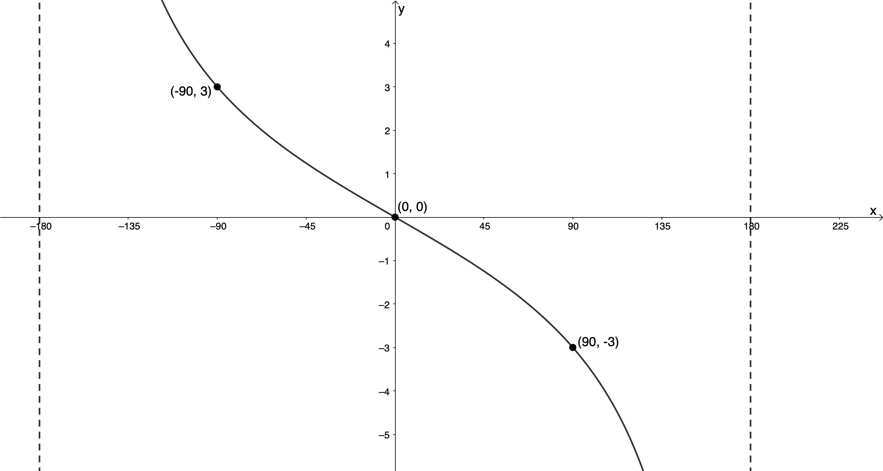
- The asymptotes within the interval are at [latex]\scriptsize x=-{{180}^\circ}[/latex] and [latex]\scriptsize x={{180}^\circ}[/latex].
- Domain: [latex]\scriptsize \{x|x\in \mathbb{R},\text{ }-{{180}^\circ} \lt x \lt {{180}^\circ}\}[/latex]
Range[latex]\scriptsize \{f(x)|f(x)\in \mathbb{R}\}\text{ }[/latex] - The period is [latex]\scriptsize {{360}^\circ}[/latex].
Exercise 11.2
Sketch the following functions for the indicated intervals:
- [latex]\scriptsize y=-2\tan \displaystyle \frac{\theta }{2}[/latex] for [latex]\scriptsize -{{180}^\circ}\le \theta \le {{180}^\circ}[/latex]
- [latex]\scriptsize \displaystyle y=\tan \left( {-\displaystyle \frac{{3x}}{2}} \right)[/latex] for [latex]\scriptsize -{{90}^\circ}\le x\le {{90}^\circ}[/latex]
- [latex]\scriptsize y=\displaystyle \frac{1}{2}\tan 3\theta[/latex] for [latex]\scriptsize {{0}^\circ}\le \theta \le {{180}^\circ}[/latex]
The full solutions are at the end of the unit.
Find the equation of a tangent function of the form [latex]\scriptsize y=a\tan kx[/latex]
By examining the location of the ‘anchor points’ and period of a graph of the form [latex]\scriptsize y=a\tan kx[/latex], we can determine the values of [latex]\scriptsize a[/latex] and [latex]\scriptsize k[/latex].
Example 11.4
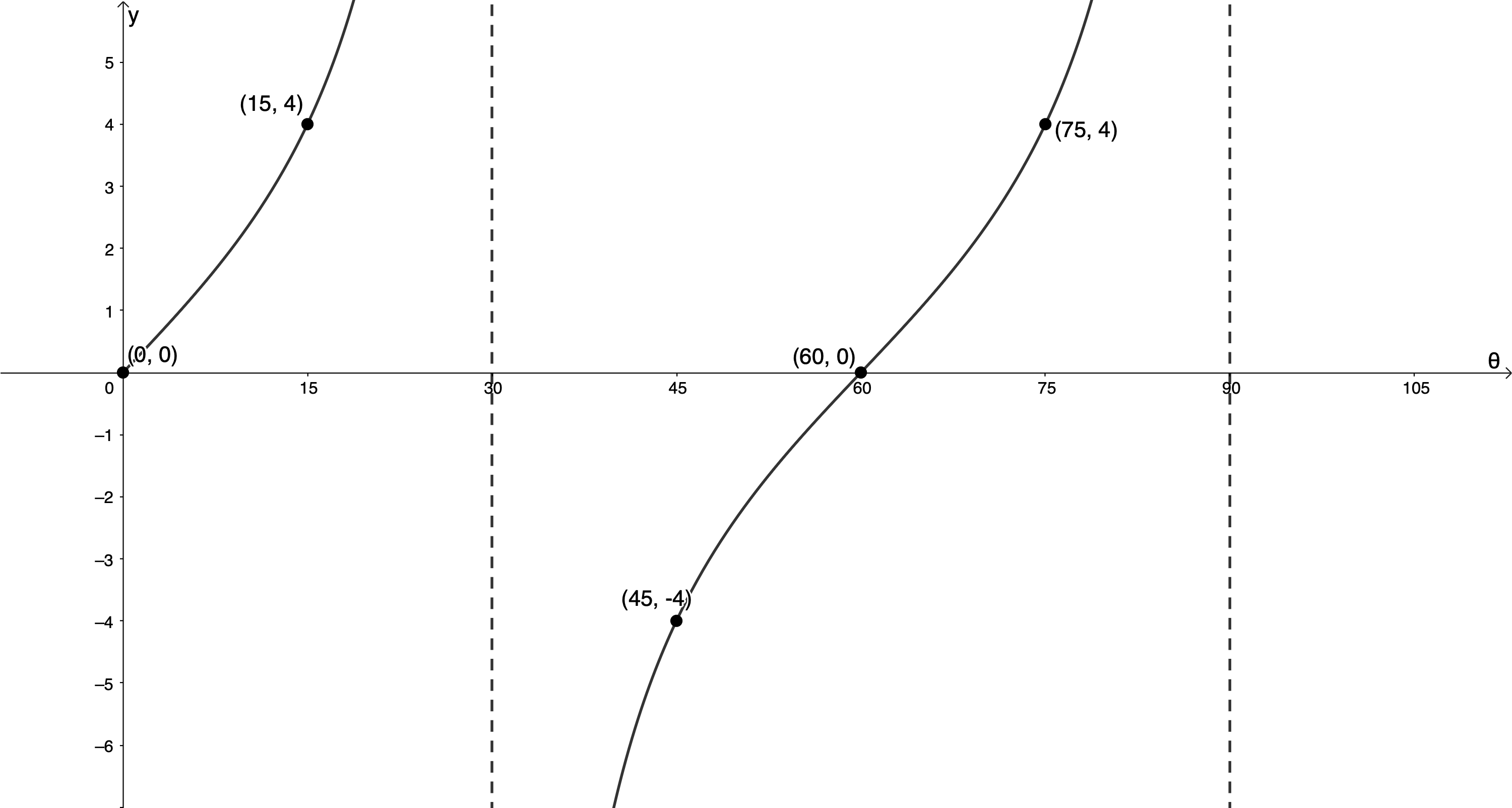
Given the following graph of the form [latex]\scriptsize y=a\cos kx[/latex], determine the values of [latex]\scriptsize a[/latex] and [latex]\scriptsize k[/latex].
Solution
From the graph we can see that the ‘anchor points’ have y-values of [latex]\scriptsize 4[/latex]. We can also see that the graph is not reflected about the x-axis. It increases to infinity as it approaches the asymptote from the left just like [latex]\scriptsize y=\tan x[/latex]. Therefore, [latex]\scriptsize a=4[/latex] and [latex]\scriptsize y=4\tan kx[/latex].
The period is [latex]\scriptsize {{60}^\circ}[/latex].
[latex]\scriptsize \begin{align*}\text{Period}&=\displaystyle \frac{{{{{180}}^\circ}}}{{\left| k \right|}}\text{ }\\{{60}^\circ}&=\displaystyle \frac{{{{{180}}^\circ}}}{{\left| k \right|}}\\\therefore \left| k \right|&=3\end{align*}[/latex]
[latex]\scriptsize y=4\tan 3x[/latex]
Example 11.5
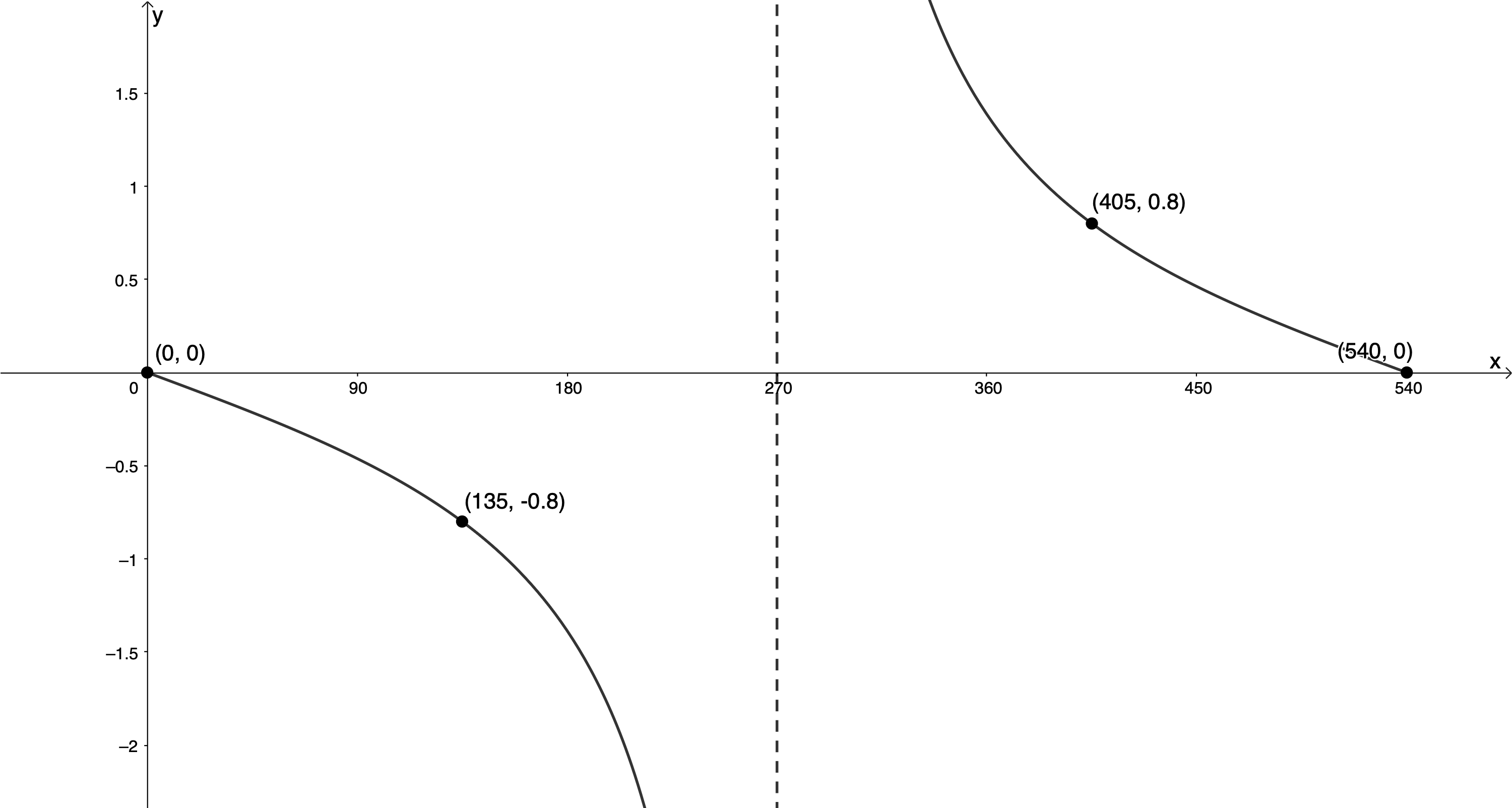
Given the following graph of the form [latex]\scriptsize y=a\tan kx[/latex], determine the values of [latex]\scriptsize a[/latex] and [latex]\scriptsize k[/latex].
Solution
From the graph we can see that the y-values of the ‘anchor points’ are [latex]\scriptsize 0.8=\displaystyle \frac{4}{5}[/latex]. We can also see that the graph is reflected about the x-axis. The function decreases to negative infinity as it approaches the asymptote from the left unlike the graph of [latex]\scriptsize \displaystyle y=\tan x[/latex], which increases to positive infinity as it approaches the asymptote from the left. Therefore, [latex]\scriptsize a=-\displaystyle \frac{4}{5}[/latex] and [latex]\scriptsize y=-\displaystyle \frac{4}{5}\tan kx[/latex].
[latex]\scriptsize \begin{align*}\text{Period}=\displaystyle \frac{{{{{180}}^\circ}}}{{\left| k \right|}}\\{{540}^\circ}=\displaystyle \frac{{{{{180}}^\circ}}}{{\left| k \right|}}\\\therefore \left| k \right|=\displaystyle \frac{{{{{180}}^\circ}}}{{{{{540}}^\circ}}}=\displaystyle \frac{1}{3}\end{align*}[/latex]
[latex]\scriptsize y=-\displaystyle \frac{4}{5}\tan \left( {\displaystyle \frac{1}{3}x} \right)[/latex]
Note: We could have assigned the negative sign to the value of [latex]\scriptsize k[/latex] but it is more common to keep [latex]\scriptsize k \gt 0[/latex] if the graph is reflected about the x-axis and make [latex]\scriptsize a \lt 0[/latex].
Exercise 11.3
Given the graph of the form [latex]\scriptsize y=a\tan kx[/latex]:
- Determine the values of [latex]\scriptsize a[/latex] and [latex]\scriptsize k[/latex].
- State the domain and range of the function.
The full solutions are at the end of the unit.
Summary
In this unit you have learnt the following:
- The effects of [latex]\scriptsize a[/latex] and [latex]\scriptsize k[/latex] on the tangent graph of the form [latex]\scriptsize y=a\tan k\theta[/latex].
- How to sketch functions of the form[latex]\scriptsize y=a\tan k\theta[/latex].
- How to find the values of [latex]\scriptsize a[/latex] and [latex]\scriptsize k[/latex] from a given tangent graph of the form[latex]\scriptsize y=a\tan k\theta[/latex].
Unit 11: Assessment
Suggested time to complete: 45 minutes
- Sketch the following functions for the given intervals:
- [latex]\scriptsize 2y=\tan \left( {-\displaystyle \frac{1}{3}x} \right)[/latex] for [latex]\scriptsize -{{270}^\circ}\le x\le {{270}^\circ}[/latex]
- [latex]\scriptsize g(x)=-3\tan 2x[/latex] for [latex]\scriptsize {{0}^\circ}\le x\le {{135}^\circ}[/latex]
- From the graph below of the form [latex]\scriptsize y=a\tan kx[/latex], determine the values of [latex]\scriptsize a[/latex] and [latex]\scriptsize k[/latex].
The full solutions are at the end of the unit.
Unit 11: Solutions
Exercise 11.1
- .
- [latex]\scriptsize y=\tan (2x)[/latex]
[latex]\scriptsize k=2[/latex]
[latex]\scriptsize \text{Period}=\displaystyle \frac{{{{{180}}^\circ}}}{{\left| 2 \right|}}=\displaystyle \frac{{{{{180}}^\circ}}}{2}={{90}^\circ}[/latex]
[latex]\scriptsize \text{Asymptote}=\displaystyle \frac{{{{{90}}^\circ}}}{{\left| k \right|}}=\displaystyle \frac{{{{{90}}^\circ}}}{2}={{45}^\circ}[/latex]
All the new asymptotes can be found by adding or subtracting multiples of the new period.
Asymptotes: [latex]\scriptsize {{45}^\circ}\pm m{{.90}^\circ},m\in \mathbb{Z}\text{ }[/latex] - [latex]\scriptsize y=\tan \left( {-\displaystyle \frac{3}{5}x} \right)[/latex]
[latex]\scriptsize k=-\displaystyle \frac{3}{5}[/latex]
[latex]\scriptsize \text{Period}=\displaystyle \frac{{{{{180}}^\circ}}}{{\left| {-\displaystyle \frac{3}{5}} \right|}}=\displaystyle \frac{{{{{180}}^\circ}}}{{\displaystyle \frac{3}{5}}}=\displaystyle \frac{{5\times {{{180}}^\circ}}}{3}={{300}^\circ}[/latex]
[latex]\scriptsize \text{Asymptote}=\displaystyle \frac{{{{{90}}^\circ}}}{{\left| k \right|}}=\displaystyle \frac{{{{{90}}^\circ}}}{{\displaystyle \frac{3}{5}}}={{150}^\circ}[/latex]
Asymptotes: [latex]\scriptsize {{150}^\circ}\pm m{{.90}^\circ},m\in \mathbb{Z}\text{ }[/latex] - [latex]\scriptsize y=\tan \left( {-\displaystyle \frac{3}{2}x} \right)[/latex]
[latex]\scriptsize k=-\displaystyle \frac{3}{2}[/latex]
[latex]\scriptsize \text{Period}=\displaystyle \frac{{{{{180}}^\circ}}}{{\left| {-\displaystyle \frac{3}{2}} \right|}}=\displaystyle \frac{{2\times {{{180}}^\circ}}}{3}={{120}^\circ}\text{ }[/latex]
[latex]\scriptsize \text{Asymptote}=\displaystyle \frac{{{{{90}}^\circ}}}{{\left| k \right|}}=\displaystyle \frac{{{{{90}}^\circ}}}{{\displaystyle \frac{3}{2}}}={{60}^\circ}[/latex]
Asymptotes: [latex]\scriptsize {{60}^\circ}\pm m{{.90}^\circ},m\in \mathbb{Z}\text{ }[/latex]
- [latex]\scriptsize y=\tan (2x)[/latex]
- .
- The period of the graph is [latex]\scriptsize {{360}^\circ}[/latex].
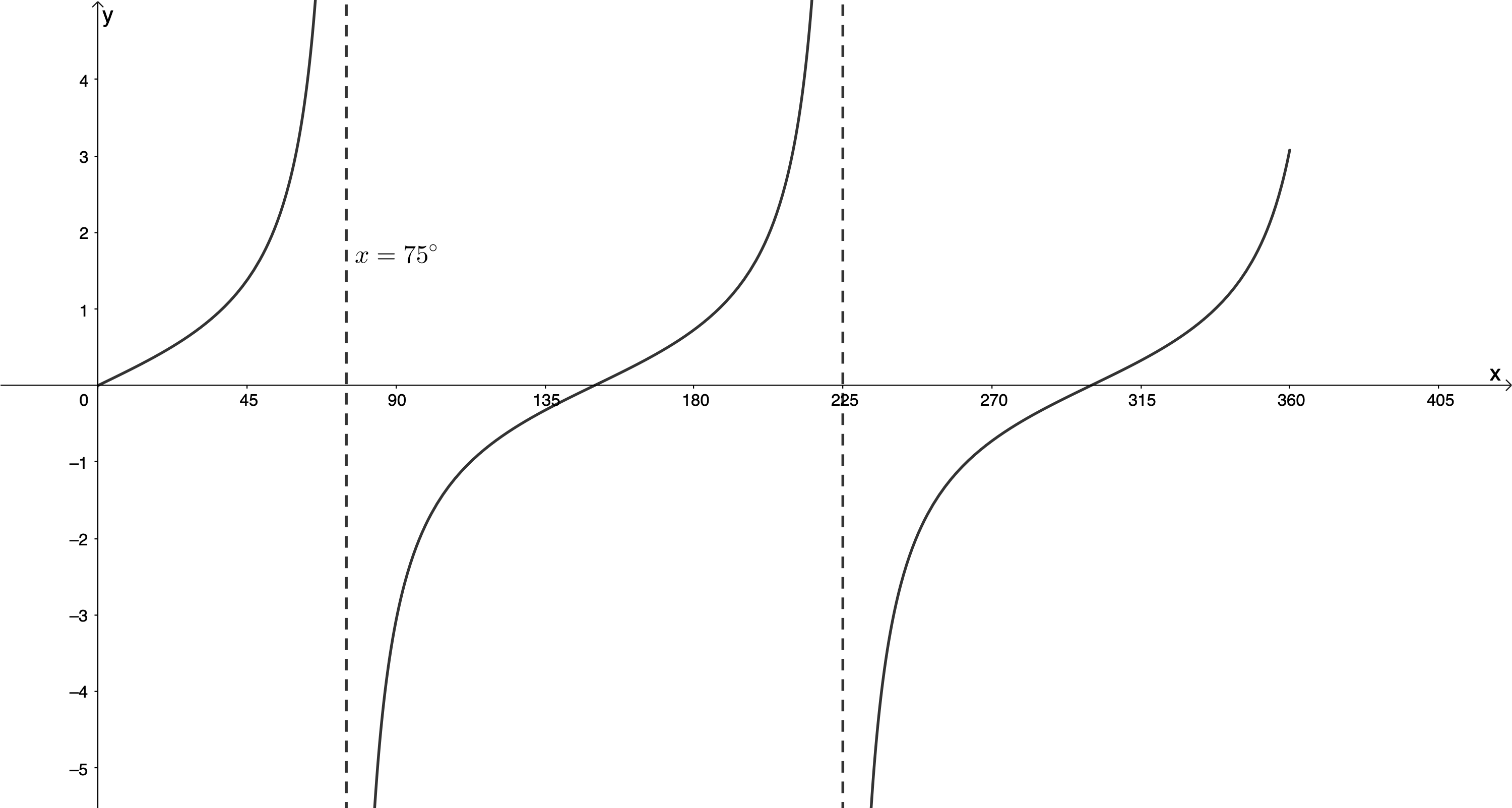
[latex]\scriptsize \begin{align*}\text{Period} & =\displaystyle \frac{{{{{180}}^\circ}}}{{\left| k \right|}}\\{{360}^\circ} & =\displaystyle \frac{{{{{180}}^\circ}}}{{\left| k \right|}}\\\therefore \left| k \right| & =\displaystyle \frac{{{{{180}}^\circ}}}{{{{{360}}^\circ}}}\\\therefore \left| k \right| & =\displaystyle \frac{1}{2}\end{align*}[/latex] - There is an asymptote at [latex]\scriptsize x={{75}^\circ}[/latex]. This means that the period is [latex]\scriptsize 2\times {{75}^\circ}={{150}^\circ}[/latex].
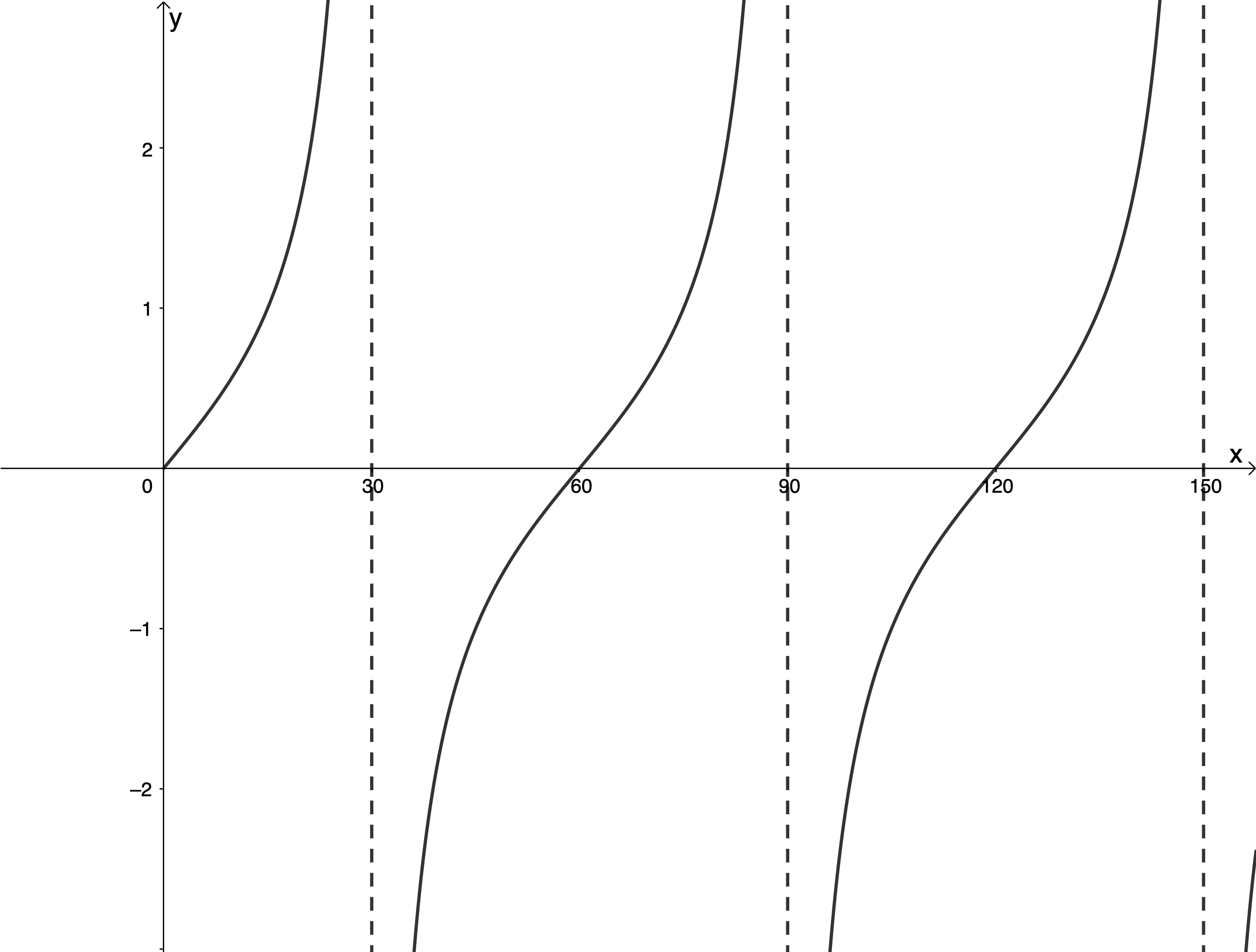
[latex]\scriptsize \displaystyle \begin{align*}\text{Period}=\displaystyle \frac{{{{{180}}^\circ}}}{{\left| k \right|}}\\{{150}^\circ}=\displaystyle \frac{{{{{180}}^\circ}}}{{\left| k \right|}}\\\therefore \left| k \right|=\displaystyle \frac{{{{{180}}^\circ}}}{{{{{150}}^\circ}}}=\displaystyle \frac{6}{5}\end{align*}[/latex] - The period of the graph is [latex]\scriptsize {{60}^\circ}[/latex].
[latex]\scriptsize \begin{align*}\text{Period}=\displaystyle \frac{{{{{180}}^\circ}}}{{\left| k \right|}}\\{{60}^\circ}=\displaystyle \frac{{{{{180}}^\circ}}}{{\left| k \right|}}\\\therefore \left| k \right|=\displaystyle \frac{{{{{180}}^\circ}}}{{{{{60}}^\circ}}}=3\end{align*}[/latex]
- The period of the graph is [latex]\scriptsize {{360}^\circ}[/latex].
Exercise 11.2
- [latex]\scriptsize y=-2\tan \displaystyle \frac{\theta }{2}[/latex] for [latex]\scriptsize -{{180}^\circ}\le \theta \le {{180}^\circ}[/latex]
[latex]\scriptsize k=\displaystyle \frac{1}{2}[/latex]
[latex]\scriptsize \text{Period}=\displaystyle \frac{{{{{180}}^\circ}}}{{\left| k \right|}}=\displaystyle \frac{{{{{180}}^\circ}}}{{\left| {\displaystyle \frac{1}{2}} \right|}}={{360}^\circ}[/latex]
[latex]\scriptsize a=-2[/latex]. Graph is reflected about the x-axis.[latex]\scriptsize \tan \theta[/latex] [latex]\scriptsize ({{0}^\circ},0)[/latex] [latex]\scriptsize ({{45}^\circ},1)[/latex] [latex]\scriptsize \theta ={{90}^\circ}[/latex] asymptote [latex]\scriptsize ({{135}^\circ},-1)[/latex] [latex]\scriptsize ({{180}^\circ},0)[/latex] [latex]\scriptsize -2\tan \left( {\displaystyle \frac{\theta }{2}} \right)[/latex] [latex]\scriptsize ({{0}^\circ},0)[/latex] [latex]\scriptsize ({{90}^\circ},-2)[/latex] [latex]\scriptsize \theta ={{180}^\circ}[/latex] asymptote [latex]\scriptsize ({{270}^\circ},2)[/latex] [latex]\scriptsize ({{360}^\circ},0)[/latex] 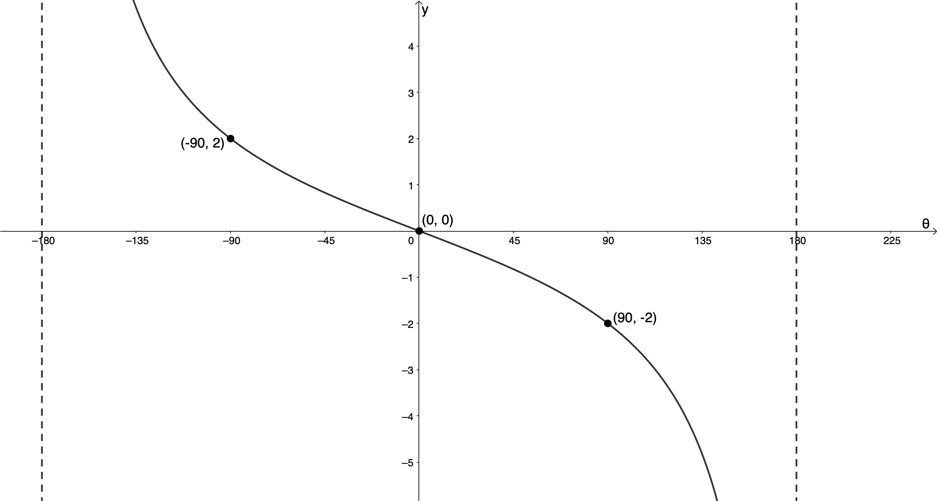
- [latex]\scriptsize y=\tan \left( {-\displaystyle \frac{{3x}}{2}} \right)[/latex] for [latex]\scriptsize -{{90}^\circ}\le x\le {{90}^\circ}[/latex]
[latex]\scriptsize k=-\displaystyle \frac{3}{2}[/latex]
[latex]\scriptsize \text{Period}=\displaystyle \frac{{{{{180}}^\circ}}}{{\left| k \right|}}=\displaystyle \frac{{{{{180}}^\circ}}}{{\left| {-\displaystyle \frac{3}{2}} \right|}}=\displaystyle \frac{{{{{180}}^\circ}}}{{\displaystyle \frac{3}{2}}}={{120}^\circ}[/latex]
[latex]\scriptsize k \lt 0[/latex], so graph is reflected about the x-axis.
[latex]\scriptsize a=1[/latex][latex]\scriptsize \tan x[/latex] [latex]\scriptsize ({{0}^\circ},0)[/latex] [latex]\scriptsize ({{45}^\circ},1)[/latex] [latex]\scriptsize x={{90}^\circ}[/latex] asymptote [latex]\scriptsize ({{135}^\circ},-1)[/latex] [latex]\scriptsize ({{180}^\circ},0)[/latex] [latex]\scriptsize \tan \left( {-\displaystyle \frac{{3x}}{2}} \right)[/latex] [latex]\scriptsize ({{0}^\circ},0)[/latex] [latex]\scriptsize ({{30}^\circ},-1)[/latex] [latex]\scriptsize x={{60}^\circ}[/latex] asymptote [latex]\scriptsize ({{90}^\circ},1)[/latex] [latex]\scriptsize ({{120}^\circ},0)[/latex] 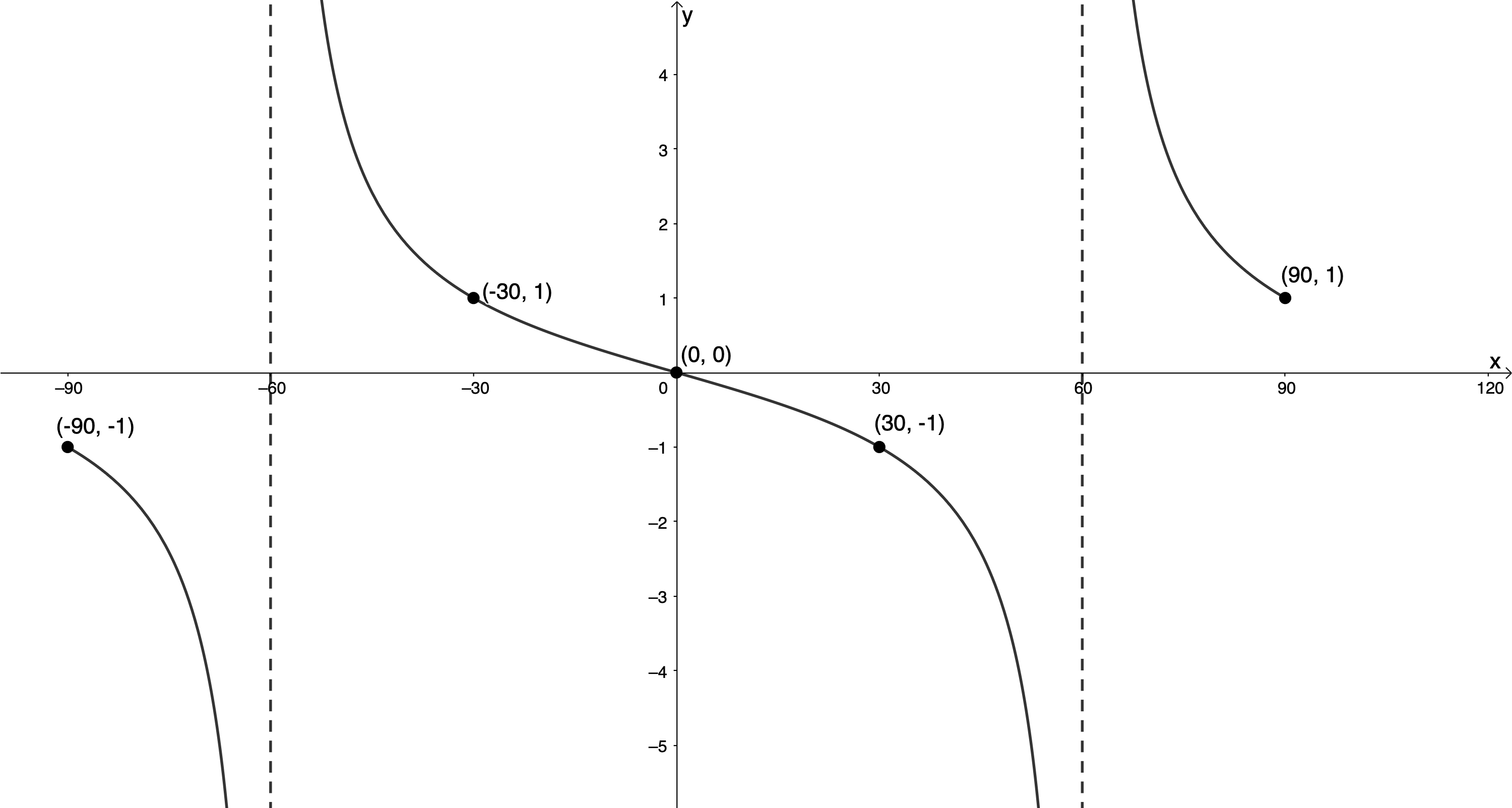
- [latex]\scriptsize y=\displaystyle \frac{1}{2}\tan 3\theta[/latex] for [latex]\scriptsize {{0}^\circ}\le x\le {{180}^\circ}[/latex]
[latex]\scriptsize k=3[/latex]
[latex]\scriptsize \text{Period}=\displaystyle \frac{{{{{180}}^\circ}}}{{\left| k \right|}}=\displaystyle \frac{{{{{180}}^\circ}}}{{\left| 3 \right|}}={{60}^\circ}\text{ }[/latex]
[latex]\scriptsize a=\displaystyle \frac{1}{2}[/latex]. Graph is not reflected about the x-axis.[latex]\scriptsize \tan \theta[/latex] [latex]\scriptsize ({{0}^\circ},0)[/latex] [latex]\scriptsize ({{45}^\circ},1)[/latex] [latex]\scriptsize \theta ={{90}^\circ}[/latex] asymptote [latex]\scriptsize ({{135}^\circ},-1)[/latex] [latex]\scriptsize ({{180}^\circ},0)[/latex] [latex]\scriptsize \displaystyle \frac{1}{2}\tan 3\theta[/latex] [latex]\scriptsize ({{0}^\circ},0)[/latex] [latex]\scriptsize ({{15}^\circ},\displaystyle \frac{1}{2})[/latex] [latex]\scriptsize \theta ={{30}^\circ}[/latex] asymptote [latex]\scriptsize ({{45}^\circ},-\displaystyle \frac{1}{2})[/latex] [latex]\scriptsize ({{60}^\circ},0)[/latex] 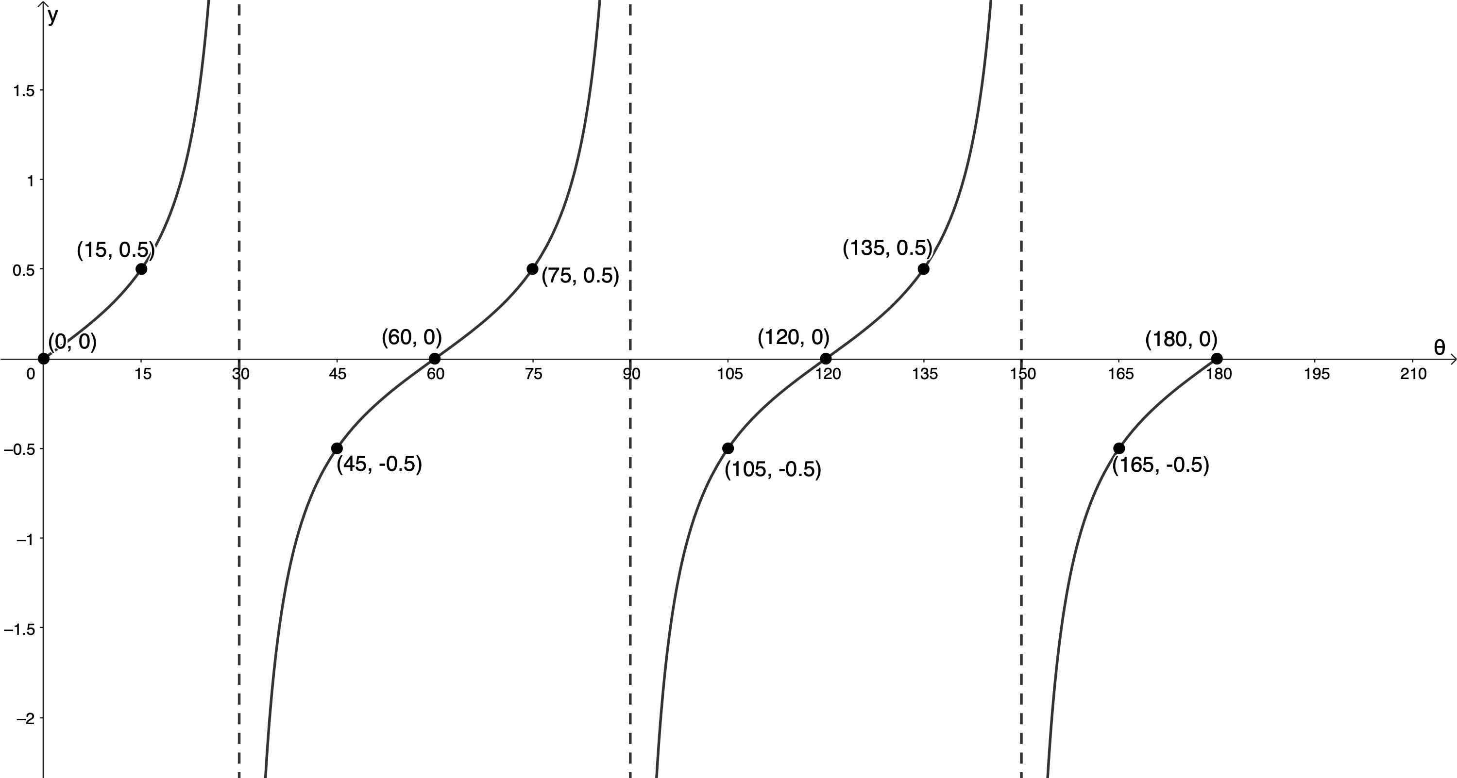
Exercise 11.3
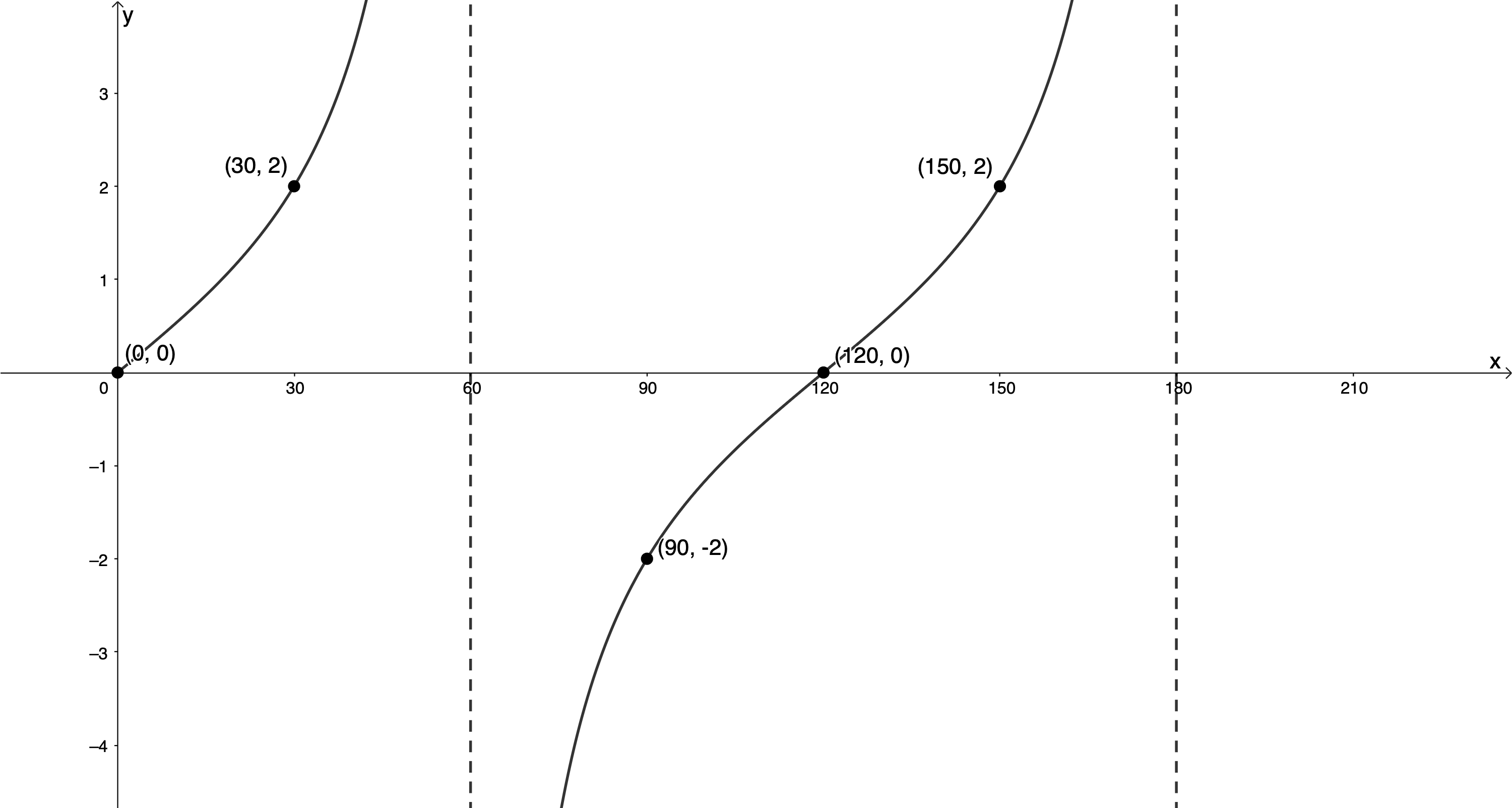
- The y-values of the ‘anchor points’ are [latex]\scriptsize 2[/latex]and the graph is not reflected about the x-axis. Therefore, [latex]\scriptsize a=2[/latex] and [latex]\scriptsize y=2\tan kx[/latex].
The period is [latex]\scriptsize {{120}^\circ}[/latex]. Therefore [latex]\scriptsize k=\displaystyle \frac{{{{{180}}^\circ}}}{{{{{120}}^\circ}}}=\displaystyle \frac{3}{2}[/latex].
[latex]\scriptsize y=2\tan \left( {\displaystyle \frac{3}{2}x} \right)[/latex] - Domain: [latex]\scriptsize \{x|x\in \mathbb{R},\text{ }{{0}^\circ}\le x \lt {{180}^\circ};x\ne 60{}^\circ \}[/latex]
Range: [latex]\scriptsize \{y|y\in \mathbb{R}\}\text{ }[/latex]
Unit 11: Assessment
- .
- [latex]\scriptsize 2y=\tan \left( {-\displaystyle \frac{1}{3}x} \right)[/latex] for [latex]\scriptsize -{{270}^\circ}\le x\le {{270}^\circ}[/latex]
[latex]\scriptsize \begin{align*}2y & =\tan \left( {-\displaystyle \frac{1}{3}x} \right)\\\therefore y & =\displaystyle \frac{1}{2}\tan \left( {-\displaystyle \frac{1}{3}x} \right)\text{ }\end{align*}[/latex]
[latex]\scriptsize k=-\displaystyle \frac{1}{3}[/latex]. Therefore, [latex]\scriptsize \text{period}=\displaystyle \frac{{{{{180}}^\circ}}}{{\left| -{\displaystyle \frac{1}{3}} \right|}}={{540}^\circ}[/latex]
[latex]\scriptsize k \lt 0[/latex]. Therefore, the graph is reflected about the x-axis.
[latex]\scriptsize a=\displaystyle \frac{1}{2}[/latex].[latex]\scriptsize \tan x[/latex] [latex]\scriptsize ({{0}^\circ},0)[/latex] [latex]\scriptsize ({{45}^\circ},1)[/latex] [latex]\scriptsize x={{90}^\circ}[/latex] asymptote [latex]\scriptsize ({{135}^\circ},-1)[/latex] [latex]\scriptsize ({{180}^\circ},0)[/latex] [latex]\scriptsize \displaystyle \frac{1}{2}\tan \left( {-\displaystyle \frac{1}{3}x} \right)[/latex] [latex]\scriptsize ({{0}^\circ},0)[/latex] [latex]\scriptsize ({{135}^\circ},-\displaystyle \frac{1}{2})[/latex] [latex]\scriptsize \displaystyle x={{270}^\circ}[/latex] asymptote [latex]\scriptsize ({{405}^\circ},\displaystyle \frac{1}{2})[/latex] [latex]\scriptsize ({{540}^\circ},0)[/latex] 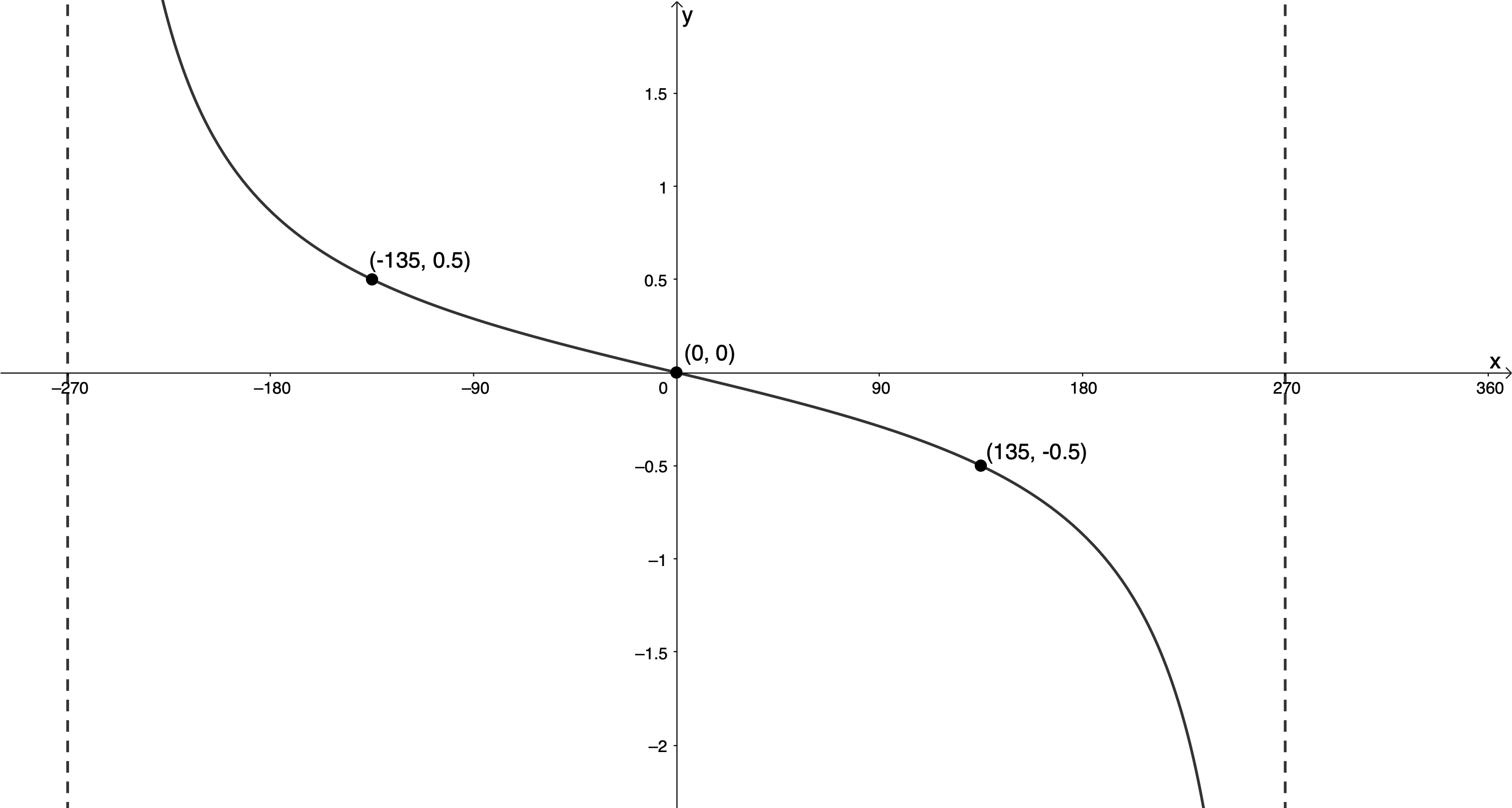
- [latex]\scriptsize g(x)=-3\tan 2x[/latex] for [latex]\scriptsize {{0}^\circ}\le x\le {{135}^\circ}[/latex]
[latex]\scriptsize k=2[/latex]. Therefore, [latex]\scriptsize \text{period}=\displaystyle \frac{{{{{180}}^\circ}}}{{\left| 2 \right|}}={{90}^\circ}[/latex]
[latex]\scriptsize a=-3[/latex]. Therefore, the graph is reflected about the x-axis.[latex]\scriptsize \tan x[/latex] [latex]\scriptsize ({{0}^\circ},0)[/latex] [latex]\scriptsize ({{45}^\circ},1)[/latex] [latex]\scriptsize x={{90}^\circ}[/latex] asymptote [latex]\scriptsize ({{135}^\circ},-1)[/latex] [latex]\scriptsize ({{180}^\circ},0)[/latex] [latex]\scriptsize -3\tan 2x[/latex] [latex]\scriptsize ({{0}^\circ},0)[/latex] [latex]\scriptsize ({{22.5}^\circ},-3)[/latex] [latex]\scriptsize \displaystyle x={{45}^\circ}[/latex] asymptote [latex]\scriptsize ({{67.5}^\circ},3)[/latex] [latex]\scriptsize ({{90}^\circ},0)[/latex] 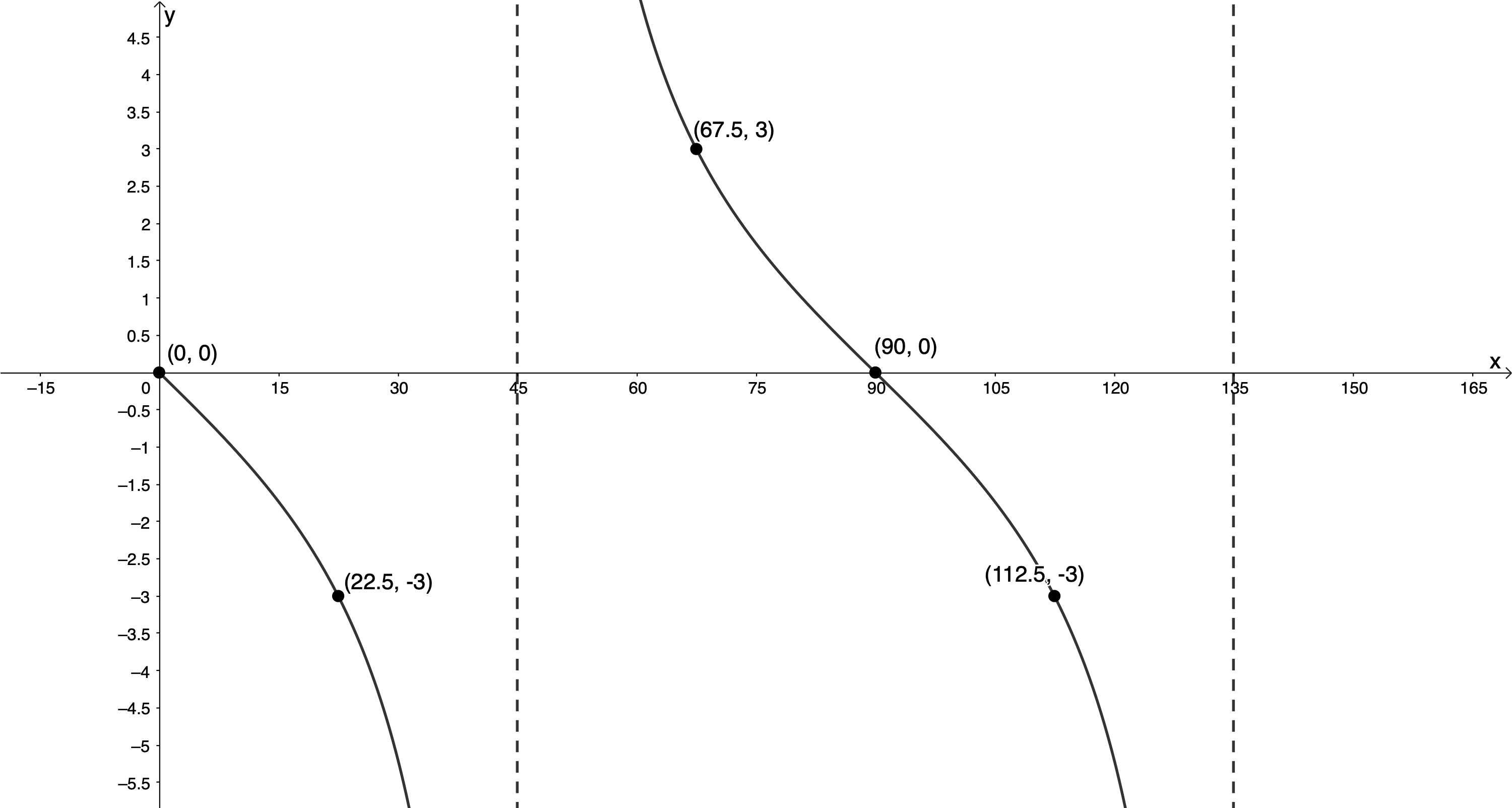
- [latex]\scriptsize 2y=\tan \left( {-\displaystyle \frac{1}{3}x} \right)[/latex] for [latex]\scriptsize -{{270}^\circ}\le x\le {{270}^\circ}[/latex]
- .
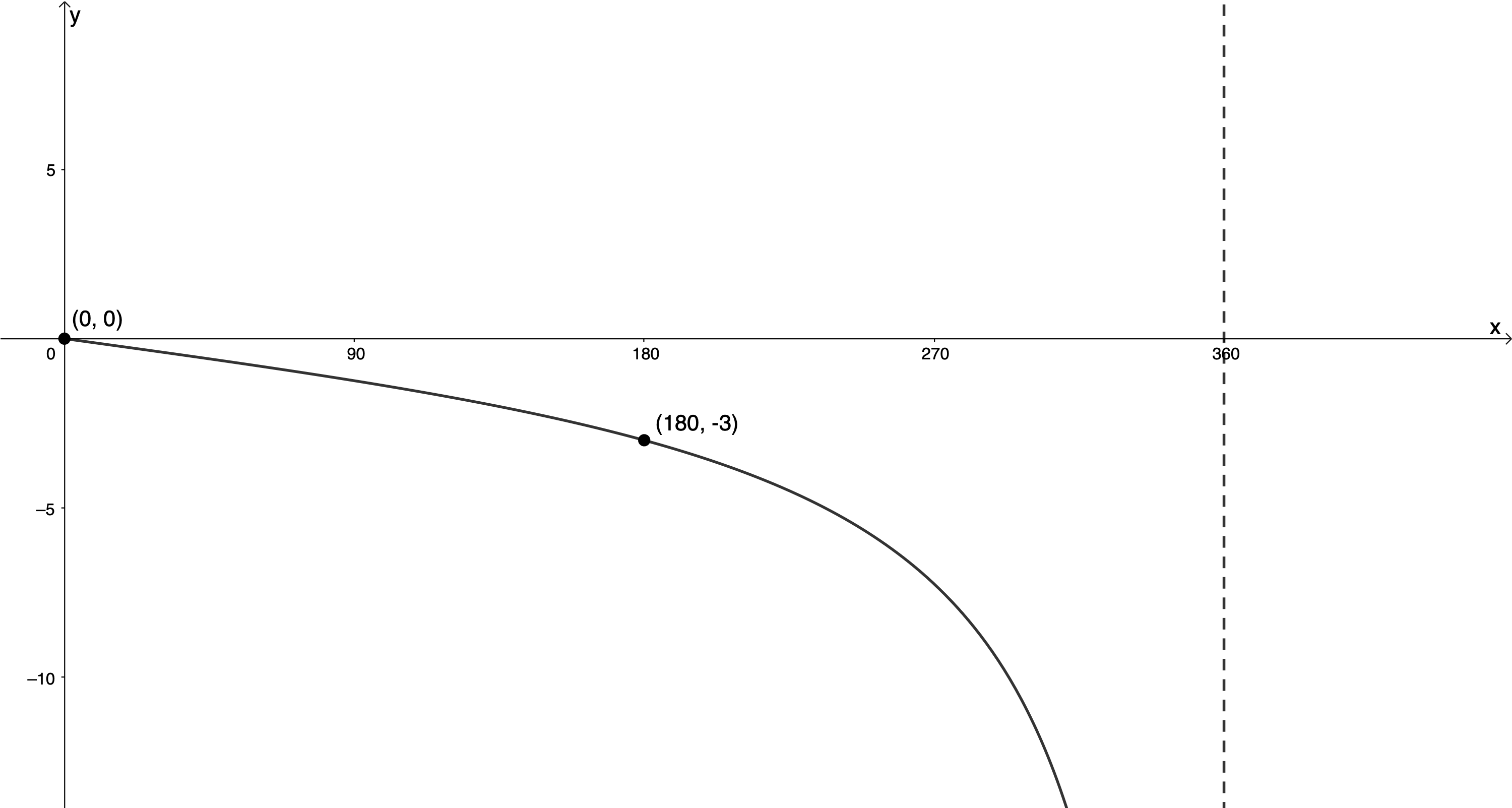
The y-value of the indicated ‘anchor point’ is [latex]\scriptsize -3[/latex] and the graph is reflected about the x-axis (it decreases to negative infinity as it approaches the asymptote from the left). Therefore, [latex]\scriptsize a=-3[/latex] and [latex]\scriptsize y=-3\tan kx[/latex].
The graph completes half a period between [latex]\scriptsize {{0}^\circ}[/latex] and [latex]\scriptsize {{360}^\circ}[/latex]. Therefore, the period is [latex]\scriptsize 2\times {{360}^\circ}={{720}^\circ}[/latex].
[latex]\scriptsize \begin{align*}\text{Period}&=\displaystyle \frac{{{{{180}}^\circ}}}{{\left| k \right|}}\\{{720}^\circ}&=\displaystyle \frac{{{{{180}}^\circ}}}{{\left| k \right|}}\\\therefore \left| k \right|&=\displaystyle \frac{{{{{180}}^\circ}}}{{{{{720}}^\circ}}}&=\displaystyle \frac{1}{4}\end{align*}[/latex]
[latex]\scriptsize y=-3\tan \left( {\displaystyle \frac{1}{4}x} \right)[/latex]
Media Attributions
- figure1 © Geogebra is licensed under a CC BY-SA (Attribution ShareAlike) license
- figure2 © Geogebra is licensed under a CC BY-SA (Attribution ShareAlike) license
- figure3 © Geogebra is licensed under a CC BY-SA (Attribution ShareAlike) license
- figure4 © DHET is licensed under a CC BY (Attribution) license
- takenote © DHET is licensed under a CC BY (Attribution) license
- exercise11.1Q2a © Geogebra is licensed under a CC BY-SA (Attribution ShareAlike) license
- exercise11.1Q2b © Geogebra is licensed under a CC BY-SA (Attribution ShareAlike) license
- exercise11.1Q2c © Geogebra is licensed under a CC BY-SA (Attribution ShareAlike) license
- figure5 © Geogebra is licensed under a CC BY-SA (Attribution ShareAlike) license
- example11.2 © Geogebra is licensed under a CC BY-SA (Attribution ShareAlike) license
- example11.3 © Geogebra is licensed under a CC BY-SA (Attribution ShareAlike) license
- example11.4 © Geogebra is licensed under a CC BY-SA (Attribution ShareAlike) license
- example11.5 © Geogebra is licensed under a CC BY-SA (Attribution ShareAlike) license
- exercise11.3 © Geogebra is licensed under a CC BY-SA (Attribution ShareAlike) license
- assessmentQ2 © Geogebra is licensed under a CC BY-SA (Attribution ShareAlike) license
- exercise11.2A1 © Geogebra is licensed under a CC BY-SA (Attribution ShareAlike) license
- exercise11.2A2 © Geogebra is licensed under a CC BY-SA (Attribution ShareAlike) license
- exercise11.2A3 © Geogebra is licensed under a CC BY-SA (Attribution ShareAlike) license
- assessmentA1a © Geogebra is licensed under a CC BY (Attribution) license
- assessmentA1b © Geogebra is licensed under a CC BY-SA (Attribution ShareAlike) license
