Functions and algebra: Use a variety of techniques to sketch and interpret information from graphs of functions
Unit 12: Horizontal transformation of the tangent graph
Dylan Busa
Unit outcomes
By the end of this unit you will be able to:
- Sketch functions of the form [latex]\scriptsize y=\tan (\theta +p)[/latex].
- Determine the effects of positive and negative values of [latex]\scriptsize p[/latex] on the tangent graph [latex]\scriptsize y=\tan (\theta +p)[/latex].
- Find the value of [latex]\scriptsize p[/latex] from a given tangent graph of the form [latex]\scriptsize y=\tan (\theta +p)[/latex].
Remember that the domain of trigonometric functions can be represented as [latex]\scriptsize x[/latex] or [latex]\scriptsize \theta[/latex]. Therefore, [latex]\scriptsize y=\tan x[/latex] and [latex]\scriptsize y=\tan \theta[/latex] are the same function.
What you should know
Before you start this unit, make sure you can:
- Sketch tangent functions of the form [latex]\scriptsize y=a\tan \theta +q[/latex]. Refer to level 2 subject outcome 2.1 Unit 5 if you need help with this.
Introduction
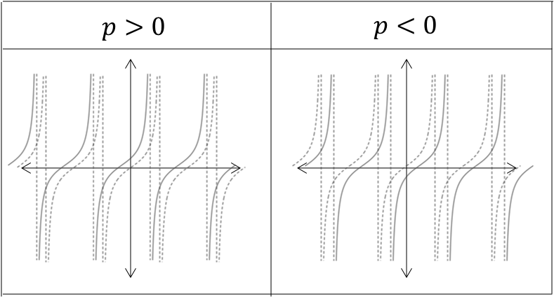
It should not surprise you that the effect of [latex]\scriptsize p[/latex] on [latex]\scriptsize y=\tan (x+p)[/latex] is also to shift the graph horizontally by [latex]\scriptsize p[/latex] units. If [latex]\scriptsize p \gt 0[/latex], the graph is shifted [latex]\scriptsize p[/latex] units to the left. If [latex]\scriptsize p \lt 0[/latex], the graph is shifted [latex]\scriptsize p[/latex] units to the right.
In the case of the sine and cosine graphs, we can track these horizontal shifts by looking at how the maximum and minimum turning points and x-intercepts are shifted, however with the tangent graph we track the vertical asymptotes, x-intercepts and other ‘anchor points’.
Take note!
In [latex]\scriptsize y=\tan (x+p)[/latex]:
- if [latex]\scriptsize p \gt 0[/latex], the graph is shifted [latex]\scriptsize p[/latex] units to the left
- if [latex]\scriptsize p \lt 0[/latex], the graph is shifted [latex]\scriptsize p[/latex] units to the right.
Note
If you have an internet connection, spend some time playing with this interactive simulation.
Here you will find a graph of the function [latex]\scriptsize \displaystyle y=\tan (x+p)[/latex] with a slider to change the value of [latex]\scriptsize p[/latex]. Pay particular attention to how changing the value of [latex]\scriptsize p[/latex] affects the location of the x-intercepts, the ‘anchor points’ and the vertical asymptotes.
Sketch functions of the form [latex]\scriptsize y=\tan (x+p)[/latex]
The best way to sketch functions of the form [latex]\scriptsize y=\tan (x+p)[/latex] is to transform the basic function of [latex]\scriptsize y=\tan x[/latex] depending on the value of [latex]\scriptsize p[/latex]. To do this, you need to know the set of ‘anchor points’ of [latex]\scriptsize y=\tan x[/latex], as transformation of these points will help you to sketch functions of the form[latex]\scriptsize y=\tan (x+p)[/latex].
Example 12.1
Given the function [latex]\scriptsize y=\tan (x+{{45}^\circ})[/latex]:
- Sketch the function for the interval [latex]\scriptsize {{0}^\circ}\le x\le {{360}^\circ}[/latex].
- State the intercepts with the axes.
- State the domain and range.
- State the period.
- State the amplitude.
Solutions
- The function is of the form [latex]\scriptsize y=\tan (x+p)[/latex] Therefore, [latex]\scriptsize p={{45}^\circ}[/latex].
.
We need to transform one period of ‘anchor points’ noting that each of these points is going to be shifted [latex]\scriptsize {{45}^\circ}[/latex] to the left.
.[latex]\scriptsize \tan x[/latex] [latex]\scriptsize ({{0}^\circ},0)[/latex] [latex]\scriptsize ({{45}^\circ},1)[/latex] [latex]\scriptsize x={{90}^\circ}[/latex] asymptote [latex]\scriptsize ({{135}^\circ},-1)[/latex] [latex]\scriptsize ({{180}^\circ},0)[/latex] [latex]\scriptsize \tan (x+{{45}^\circ})[/latex] [latex]\scriptsize (-{{45}^\circ},0)[/latex] [latex]\scriptsize ({{0}^\circ},1)[/latex] [latex]\scriptsize x={{45}^\circ}[/latex] asymptote [latex]\scriptsize ({{90}^\circ},-1)[/latex] [latex]\scriptsize ({{135}^\circ},0)[/latex] To make sure that the shape of the graph is as accurate as possible, we must also find the y-intercept.
y-intercept (let [latex]\scriptsize x=0[/latex]):
[latex]\scriptsize \begin{align*}y & =\tan ({{0}^\circ}+{{45}^\circ})\\\therefore y & =1\end{align*}[/latex]
.
Because the period of the function is [latex]\scriptsize {{180}^\circ}[/latex] we know that the function value at [latex]\scriptsize {{180}^\circ}[/latex] will also be [latex]\scriptsize 1[/latex].
.
We can now plot our transformed ‘anchor points’ and draw the graph for the interval [latex]\scriptsize {{0}^\circ}\le x\le {{360}^\circ}[/latex].
.
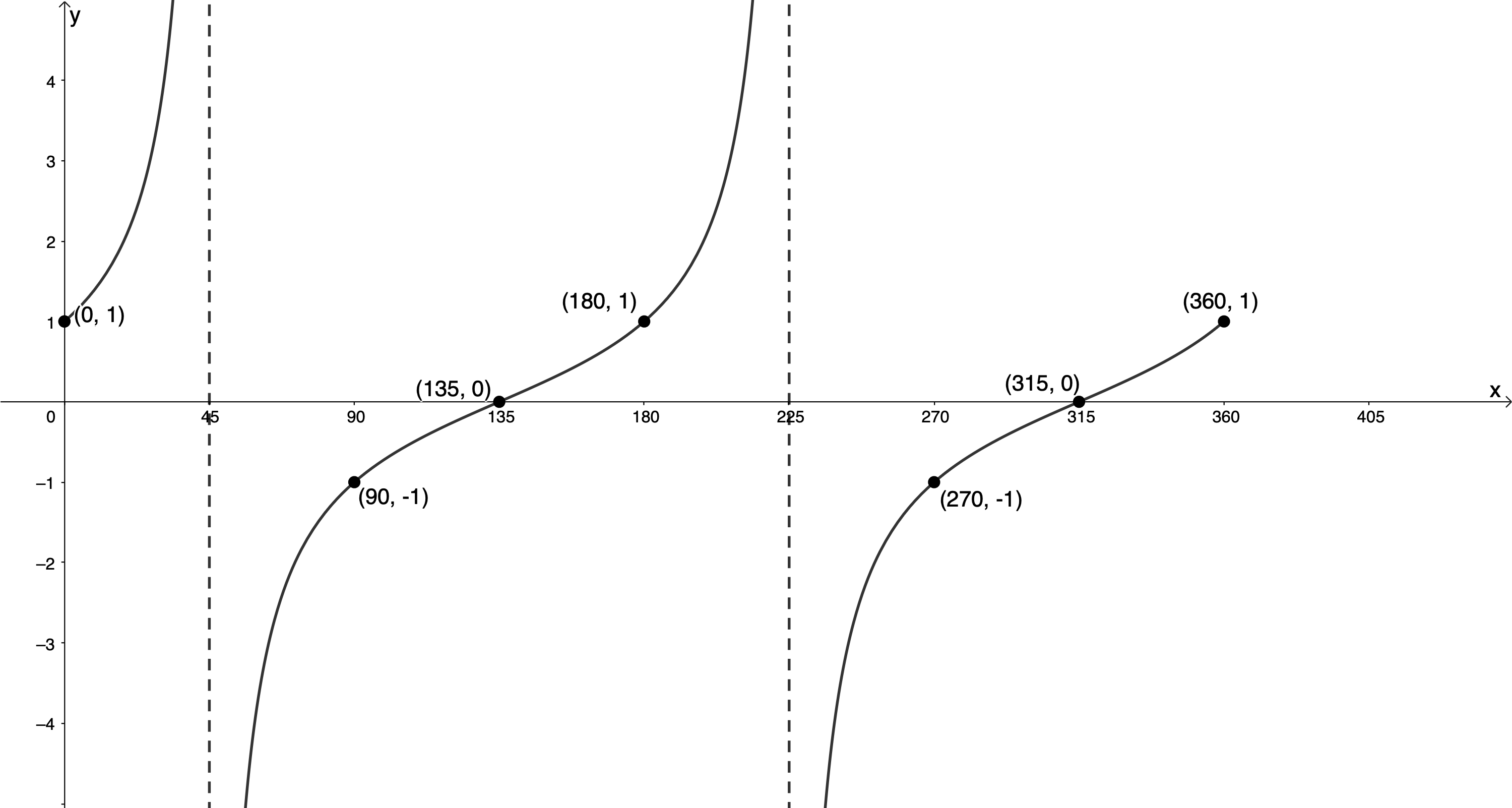
- y-intercept: [latex]\scriptsize ({{0}^\circ},1)[/latex]
x-intercepts: [latex]\scriptsize ({{135}^\circ},0)[/latex] and [latex]\scriptsize ({{315}^\circ},0)[/latex] - Domain: [latex]\scriptsize \{x|x\in \mathbb{R},\text{ }{{0}^\circ}\le x\le {{360}^\circ};x\ne 45{}^\circ ,225{}^\circ \}[/latex]
Range: [latex]\scriptsize \{y|y\in \mathbb{R}\}\text{ }[/latex] - The period is [latex]\scriptsize {{180}^\circ}[/latex].
- The amplitude is undefined because the tangent graph increases to positive and negative infinity at the asymptotes.
Take note!
In general, the domain of the function [latex]\scriptsize y=\tan (x+p)[/latex] is [latex]\scriptsize x\in \mathbb{R}\text{ }[/latex], excluding the x-values of the asymptotes. We had to restrict the domain in Example 12.1, because the interval in which we were working was restricted.
Exercise 12.1
Sketch the following functions for the indicated intervals on separate sets of axes:
- [latex]\scriptsize f(x)=\tan (x+{{30}^\circ})[/latex] for [latex]\scriptsize {{0}^\circ}\le x\le {{360}^\circ}[/latex]
- [latex]\scriptsize g(x)=\tan (x-{{45}^\circ})[/latex] for [latex]\scriptsize -{{180}^\circ}\le x\le {{180}^\circ}[/latex]
- [latex]\scriptsize h(x)=\tan (x-{{40}^\circ})[/latex] for [latex]\scriptsize -{{180}^\circ}\le x\le {{180}^\circ}[/latex]
The full solutions are at the end of the unit.
Sketch functions of the form [latex]\scriptsize y=a\tan (x+p)[/latex]
Now that we know that the value of [latex]\scriptsize p[/latex] shifts the function of the form [latex]\scriptsize y=\tan (x+p)[/latex] horizontally by [latex]\scriptsize p[/latex] degrees, we can combine this with our knowledge of the effects of [latex]\scriptsize a[/latex], and examine functions of the form [latex]\scriptsize y=a\tan (x+p)[/latex].
Example 12.2
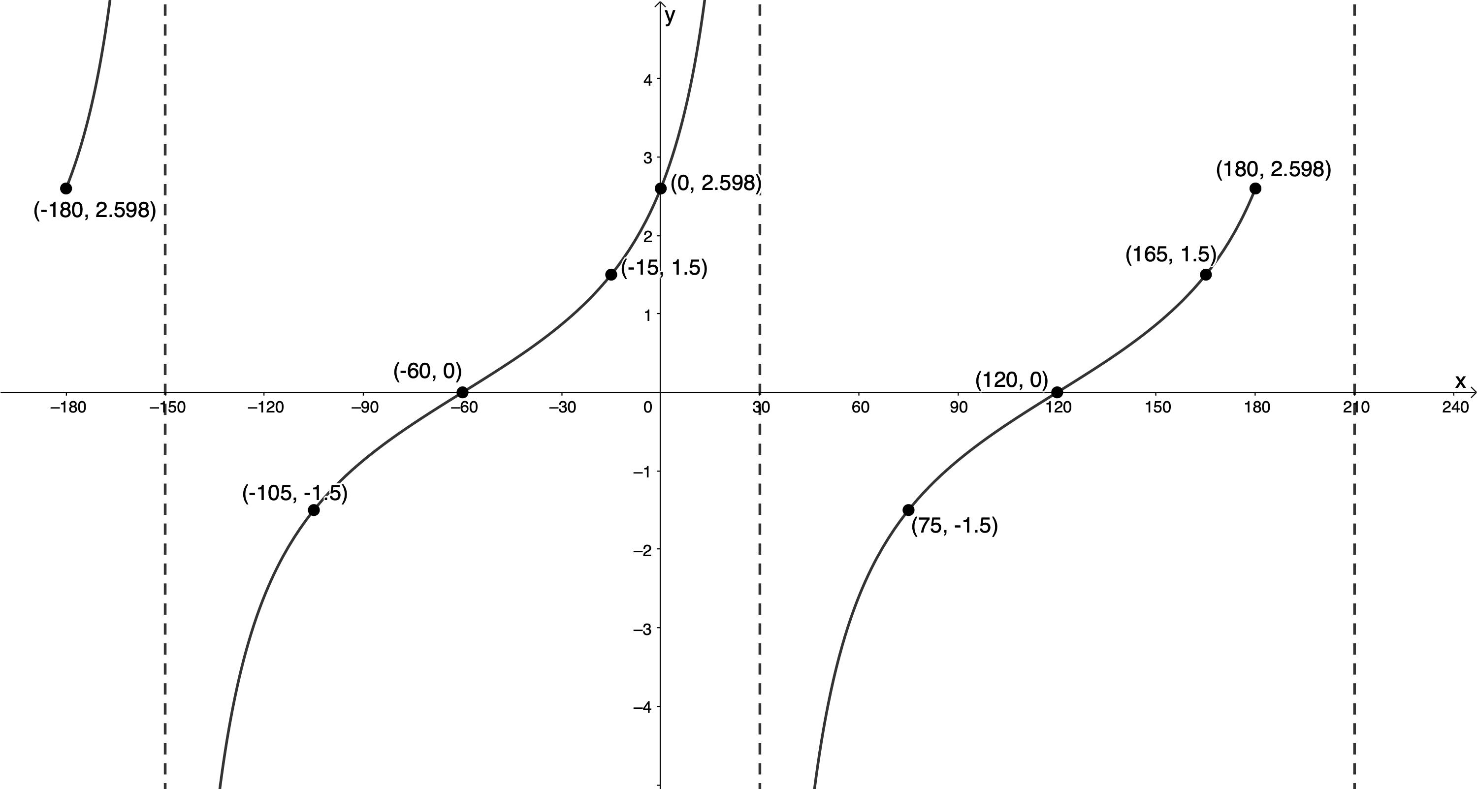
Sketch the graph of [latex]\scriptsize f(x)=1.5\tan (x+{{60}^\circ})[/latex] for the interval [latex]\scriptsize -{{180}^\circ}\le x\le {{180}^\circ}[/latex].
Solution
The function is of the form [latex]\scriptsize y=a\tan (x+p)[/latex] where [latex]\scriptsize a=1.5[/latex] and [latex]\scriptsize p={{60}^\circ}[/latex].
We need to transform one period of ‘anchor points’ noting that each of these points is going to be shifted [latex]\scriptsize {{60}^\circ}[/latex] to the left and each of the y-values is going to be multiplied by [latex]\scriptsize 1.5[/latex].
| [latex]\scriptsize \tan x[/latex] | [latex]\scriptsize ({{0}^\circ},0)[/latex] | [latex]\scriptsize ({{45}^\circ},1)[/latex] | [latex]\scriptsize x={{90}^\circ}[/latex] asymptote | [latex]\scriptsize ({{135}^\circ},-1)[/latex] | [latex]\scriptsize ({{180}^\circ},0)[/latex] |
| [latex]\scriptsize 1.5\tan (x+{{60}^\circ})[/latex] | [latex]\scriptsize (-{{60}^\circ},0)[/latex] | [latex]\scriptsize (-{{15}^\circ},1.5)[/latex] | [latex]\scriptsize x={{30}^\circ}[/latex] asymptote | [latex]\scriptsize ({{75}^\circ},-1.5)[/latex] | [latex]\scriptsize ({{120}^\circ},0)[/latex] |
To make sure that the shape of the graph is as accurate as possible, we must also find the y-intercept.
y-intercept (let [latex]\scriptsize x=0[/latex]):
[latex]\scriptsize \begin{align*}y & =1.5\tan ({{0}^\circ}+{{60}^\circ})\text{ }\\\therefore y & =1.5\times \displaystyle \frac{{\sqrt{3}}}{1}=\displaystyle \frac{{3\sqrt{3}}}{2}\\&=2.598\end{align*}[/latex]
Because the period of the function is [latex]\scriptsize {{180}^\circ}[/latex] we know that the function values at [latex]\scriptsize -{{180}^\circ}[/latex] and [latex]\scriptsize {{180}^\circ}[/latex] will also be [latex]\scriptsize 2.598[/latex].
We can now plot our transformed ‘anchor points’ and draw the graph for the interval [latex]\scriptsize -{{180}^\circ}\le x\le {{180}^\circ}[/latex].
Example 12.3
Given the function [latex]\scriptsize f(x)=2\tan ({{30}^\circ}-x)[/latex]:
- Sketch the graph for the interval [latex]\scriptsize {{0}^\circ}\le x\le {{180}^\circ}[/latex].
- State the intercepts with the axes.
- State the domain and range.
- State the amplitude and period.
Solutions
- The function is not in the form [latex]\scriptsize y=a\tan (x+p)[/latex]. We first need to get it into this form.
[latex]\scriptsize \begin{align*}f(x)&=2\tan ({{30}^\circ}-x)\\&=2\tan (-x+{{30}^\circ})\\&=2\tan \left( {-\left( {x-{{{30}}^\circ}} \right)} \right)\\&=-2\tan (x-{{30}^\circ})\end{align*}[/latex]
.
We know from the previous unit that [latex]\scriptsize \tan (-x)=-\tan (x)[/latex]. In other words, the graph of [latex]\scriptsize f(x)=\tan ({{30}^\circ}-x)[/latex] is going to be a reflection of the standard tangent graph about the x-axis because [latex]\scriptsize a=-1[/latex].
.
We need to transform one period of ‘anchor points’ noting that each of these points is going to be shifted [latex]\scriptsize {{30}^\circ}[/latex] to the right and each of the y-values of these points needs to be multiplied by [latex]\scriptsize -2[/latex].
.[latex]\scriptsize \tan x[/latex] [latex]\scriptsize ({{0}^\circ},0)[/latex] [latex]\scriptsize ({{45}^\circ},1)[/latex] [latex]\scriptsize x={{90}^\circ}[/latex] asymptote [latex]\scriptsize ({{135}^\circ},-1)[/latex] [latex]\scriptsize ({{180}^\circ},0)[/latex] [latex]\scriptsize -2\tan (x-{{30}^\circ})[/latex] [latex]\scriptsize ({{30}^\circ},0)[/latex] [latex]\scriptsize ({{75}^\circ},-2)[/latex] [latex]\scriptsize x={{120}^\circ}[/latex] asymptote [latex]\scriptsize ({{165}^\circ},2)[/latex] [latex]\scriptsize ({{210}^\circ},0)[/latex] To make sure that the shape of the graph is as accurate as possible, we must also find the y-intercept.
y-intercept (let [latex]\scriptsize x=0[/latex]):
[latex]\scriptsize \displaystyle \begin{align*}f(0) & =-2\tan ({{0}^\circ}-{{30}^\circ})\\\therefore f(0) & =-2\times -\displaystyle \frac{1}{{\sqrt{3}}}=\displaystyle \frac{2}{{\sqrt{3}}}\\&=1.155\end{align*}[/latex]
.
Because the period of the function is [latex]\scriptsize {{180}^\circ}[/latex] we know that the function value at [latex]\scriptsize {{180}^\circ}[/latex] will also be [latex]\scriptsize 1.155[/latex].
.
We can now plot our transformed ‘anchor points’ and draw the graph for the interval [latex]\scriptsize {{0}^\circ}\le x\le {{180}^\circ}[/latex]. Remember that because [latex]\scriptsize a=-1\text{ }[/latex], the graph is reflected about the x-axis. This means that it decreases to negative infinity as it approaches the asymptote from the left and increases to positive infinity as it approaches the asymptote from the right, the opposite to the function [latex]\scriptsize y=\tan x[/latex].
.
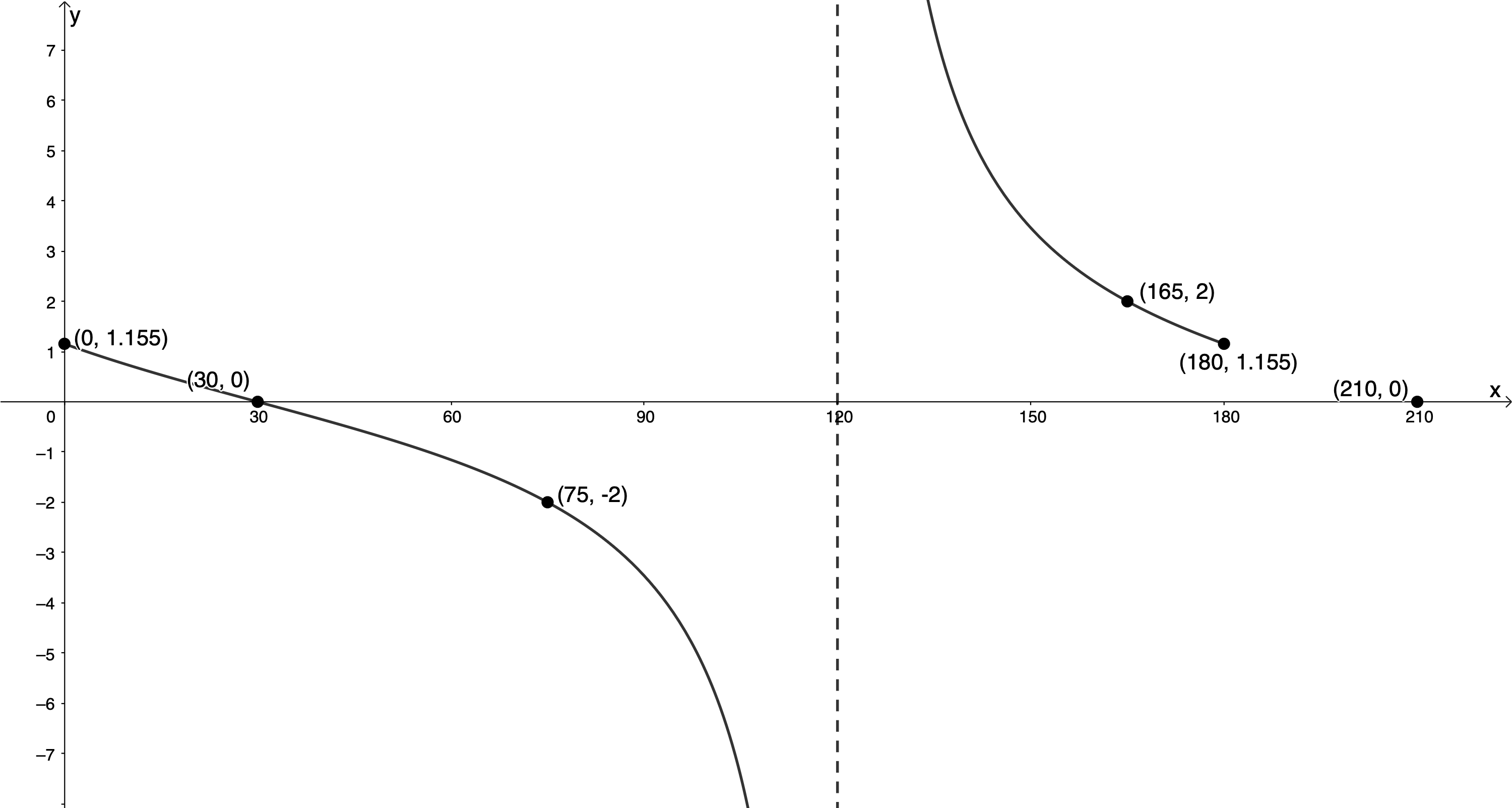
- y-intercept: [latex]\scriptsize ({{0}^\circ},\displaystyle \frac{2}{{\sqrt{3}}})\text{ }[/latex] or [latex]\scriptsize ({{0}^\circ},1.155)[/latex]
x-intercepts: [latex]\scriptsize ({{30}^\circ},0)[/latex] - Domain: [latex]\scriptsize \{x|x\in \mathbb{R},\text{ }{{0}^\circ}\le x\le {{180}^\circ};x\ne 120{}^\circ \}[/latex]
Range: [latex]\scriptsize \{f(x)|f(x)\in \mathbb{R}\}\text{ }[/latex] - The period is [latex]\scriptsize {{180}^\circ}[/latex].
The amplitude is undefined because the function values increase to positive and negative infinity as the function approaches the asymptote from the right and left respectively.
Exercise 12.2
For each of the following functions, sketch the graph for the indicated interval and state the domain and range and intercepts with the axes:
- [latex]\scriptsize y=-2\tan (x+{{45}^\circ})[/latex] for [latex]\scriptsize {{0}^\circ}\le x\le {{180}^\circ}[/latex]
- [latex]\scriptsize 2y=\tan (x-{{45}^\circ})[/latex] for [latex]\scriptsize {{0}^\circ}\le x\le {{360}^\circ}[/latex]
- [latex]\scriptsize \displaystyle \frac{1}{3}y=\tan ({{60}^\circ}-x)[/latex] for [latex]\scriptsize -{{180}^\circ}\le x\le {{180}^\circ}[/latex]
The full solutions are at the end of the unit.
Find the equation of a tangent function of the form [latex]\scriptsize y=a\tan (x+p)[/latex]
By examining the amplitude and the horizontal shift of [latex]\scriptsize y=a\tan (x+p)[/latex], we can determine the values of [latex]\scriptsize a[/latex] and [latex]\scriptsize p[/latex].
Example 12.4
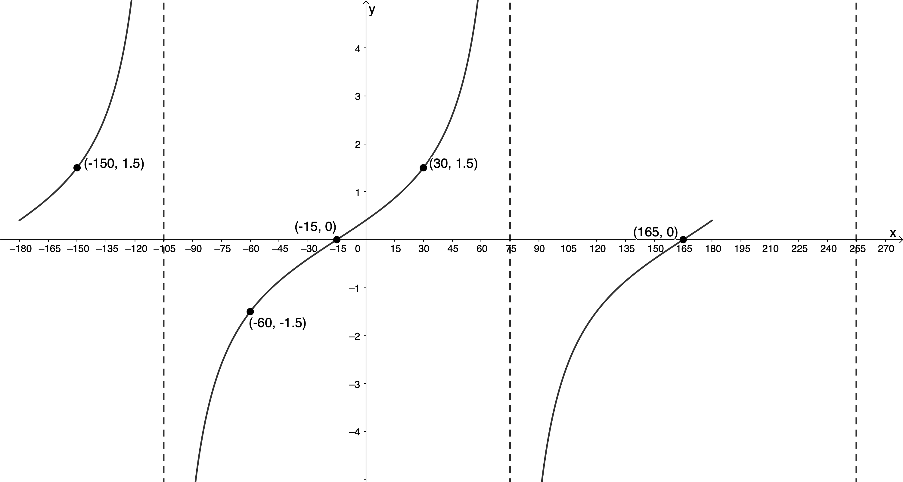
The graph below is a function of the form [latex]\scriptsize y=a\tan (x+p)[/latex]. Determine the values of [latex]\scriptsize a[/latex] and [latex]\scriptsize p[/latex].
Solution
We are told that the function is of the form [latex]\scriptsize y=a\tan (x+p)[/latex].
We know that the function [latex]\scriptsize y=\tan x[/latex] has a vertical asymptote at [latex]\scriptsize x={{90}^\circ}[/latex]. This graph has an asymptote at [latex]\scriptsize x={{75}^\circ}[/latex]. Therefore, the graph has been shifted [latex]\scriptsize {{15}^\circ}[/latex] to the left and [latex]\scriptsize p={{15}^\circ}[/latex]. The ‘anchor point’ that is normally at [latex]\scriptsize ({{45}^\circ},1)[/latex] is now at [latex]\scriptsize ({{30}^\circ},1.5)[/latex]. This confirms the fact that the graph has been shifted [latex]\scriptsize {{15}^\circ}[/latex] to the left but also tells us that [latex]\scriptsize a=1.5[/latex].
Therefore, the function is [latex]\scriptsize y=1.5\tan (x+{{15}^\circ})[/latex].
Example 12.5
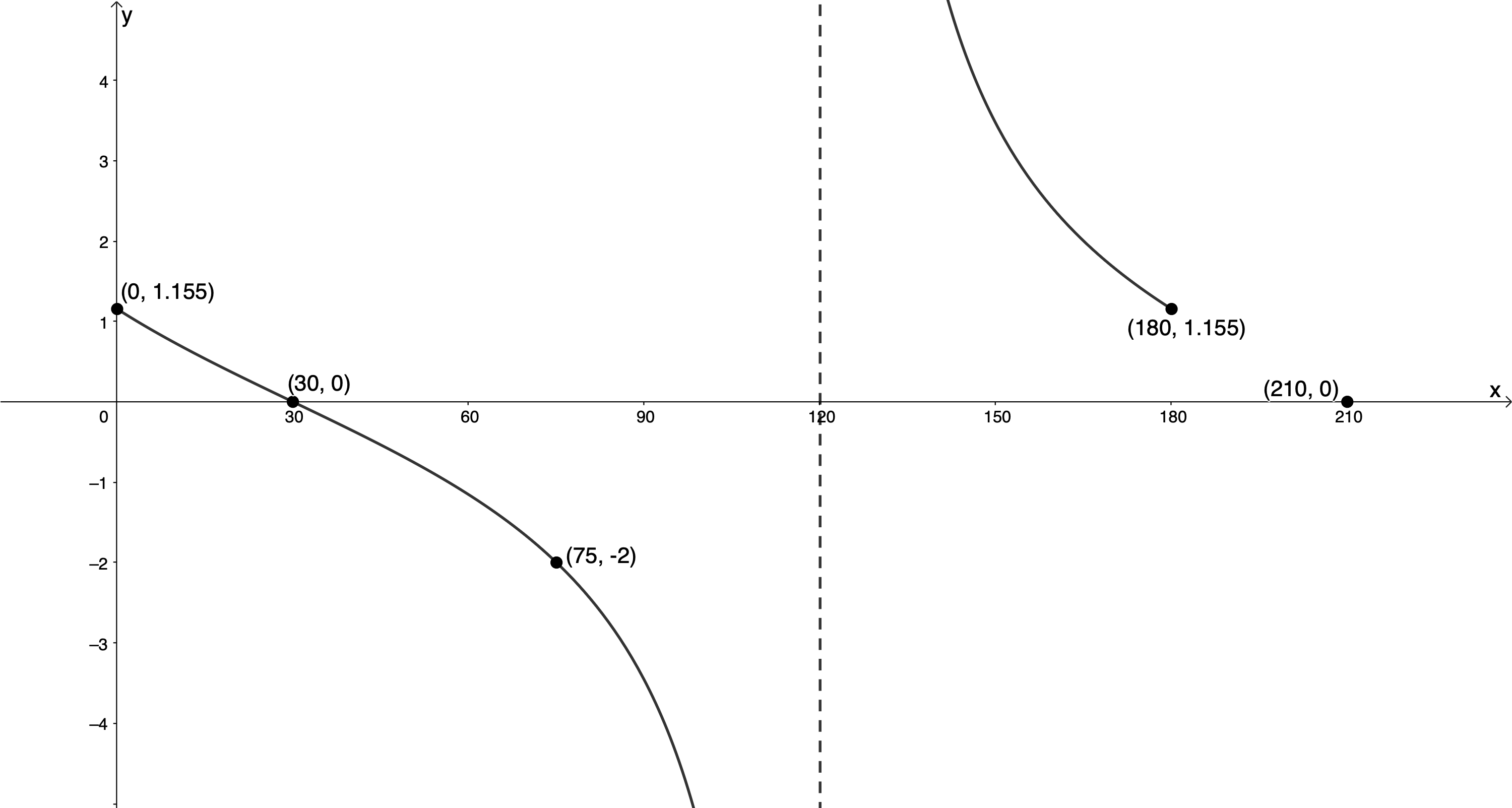
The graph below is a function of the form [latex]\scriptsize y=a\tan (x+p)[/latex]. Determine the values of [latex]\scriptsize a[/latex] and [latex]\scriptsize p[/latex].
Solution
We are told that the function is of the form [latex]\scriptsize y=a\tan (x+p)[/latex].
The asymptote that is normally at [latex]\scriptsize x={{90}^\circ}[/latex] is at [latex]\scriptsize x={{120}^\circ}[/latex]. The graph has been shifted [latex]\scriptsize {{30}^\circ}[/latex] to the right. Therefore, [latex]\scriptsize p=-{{30}^\circ}[/latex].
The anchor point that was at [latex]\scriptsize ({{45}^\circ},1)[/latex] is now at [latex]\scriptsize ({{75}^\circ},-2)[/latex]. In addition, the graph decreases to negative infinity as the function approaches the asymptote from the left. Therefore, [latex]\scriptsize a=-2[/latex].
The function is [latex]\scriptsize y=-2\tan (x-{{30}^\circ})[/latex].
Exercise 12.3
Given the graph of the form [latex]\scriptsize y=a\tan (x+p)[/latex]:
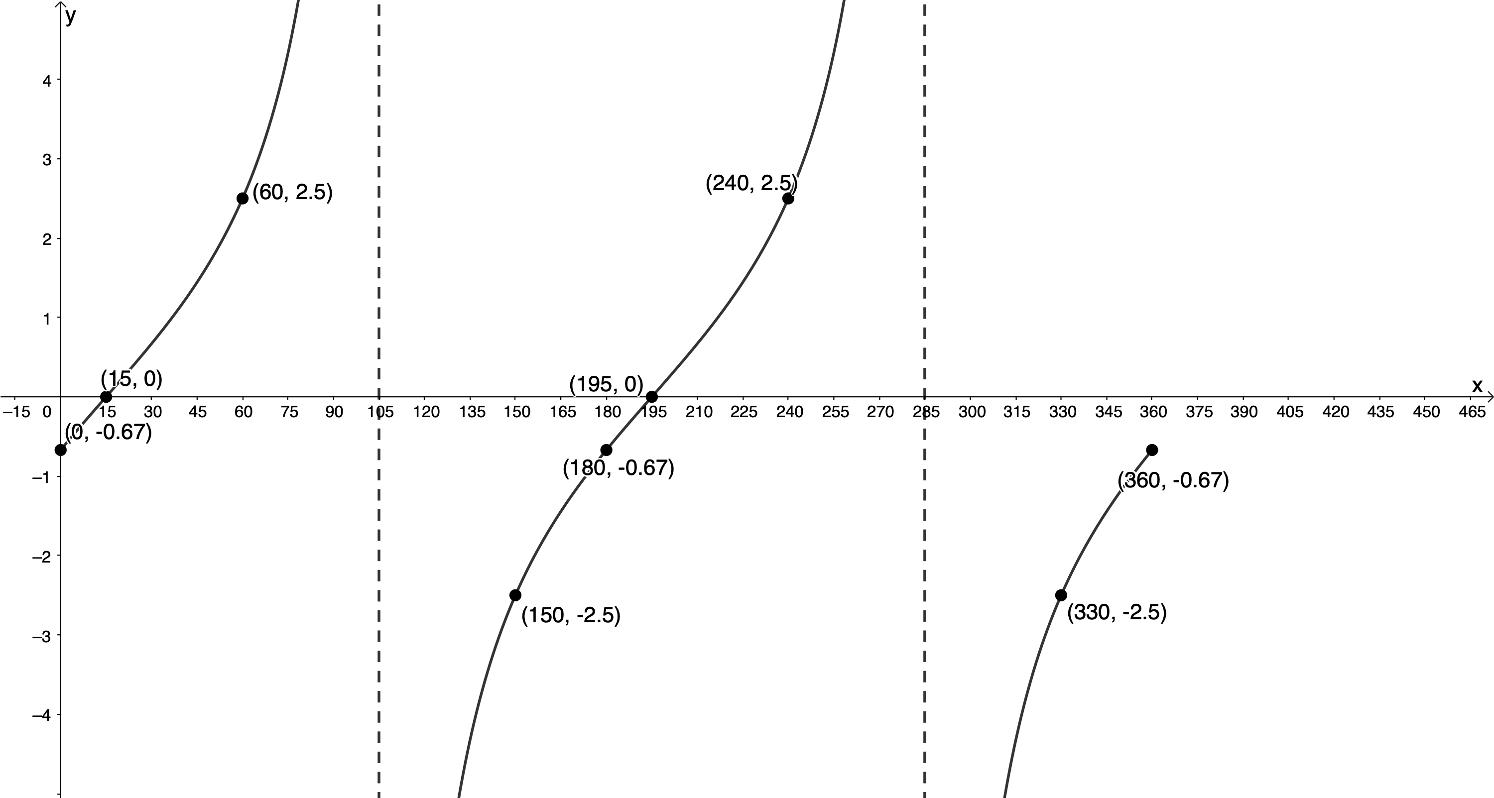
- Determine the values of [latex]\scriptsize a[/latex] and [latex]\scriptsize p[/latex].
- State the domain and range of the function.
The full solutions are at the end of the unit.
Summary
In this unit you have learnt the following:
- The effects of [latex]\scriptsize a[/latex] and [latex]\scriptsize p[/latex] on the tangent graph of the form [latex]\scriptsize y=a\tan (x+p)[/latex].
- How to sketch functions of the form [latex]\scriptsize y=a\tan (x+p)[/latex].
- How to find the values of [latex]\scriptsize a[/latex] and [latex]\scriptsize p[/latex] from a given tangent graph of the form [latex]\scriptsize y=a\tan (x+p)[/latex].
Unit 12: Assessment
Suggested time to complete: 45 minutes
- Sketch the following functions for the given intervals:
- [latex]\scriptsize 2y=-\tan \left( {x-{{{60}}^\circ}} \right)[/latex] for [latex]\scriptsize {{0}^\circ}\le x\le {{360}^\circ}[/latex]
- [latex]\scriptsize g(x)=-3\tan ({{45}^\circ}-x)[/latex] for [latex]\scriptsize -{{180}^\circ}\le x\le {{180}^\circ}[/latex]
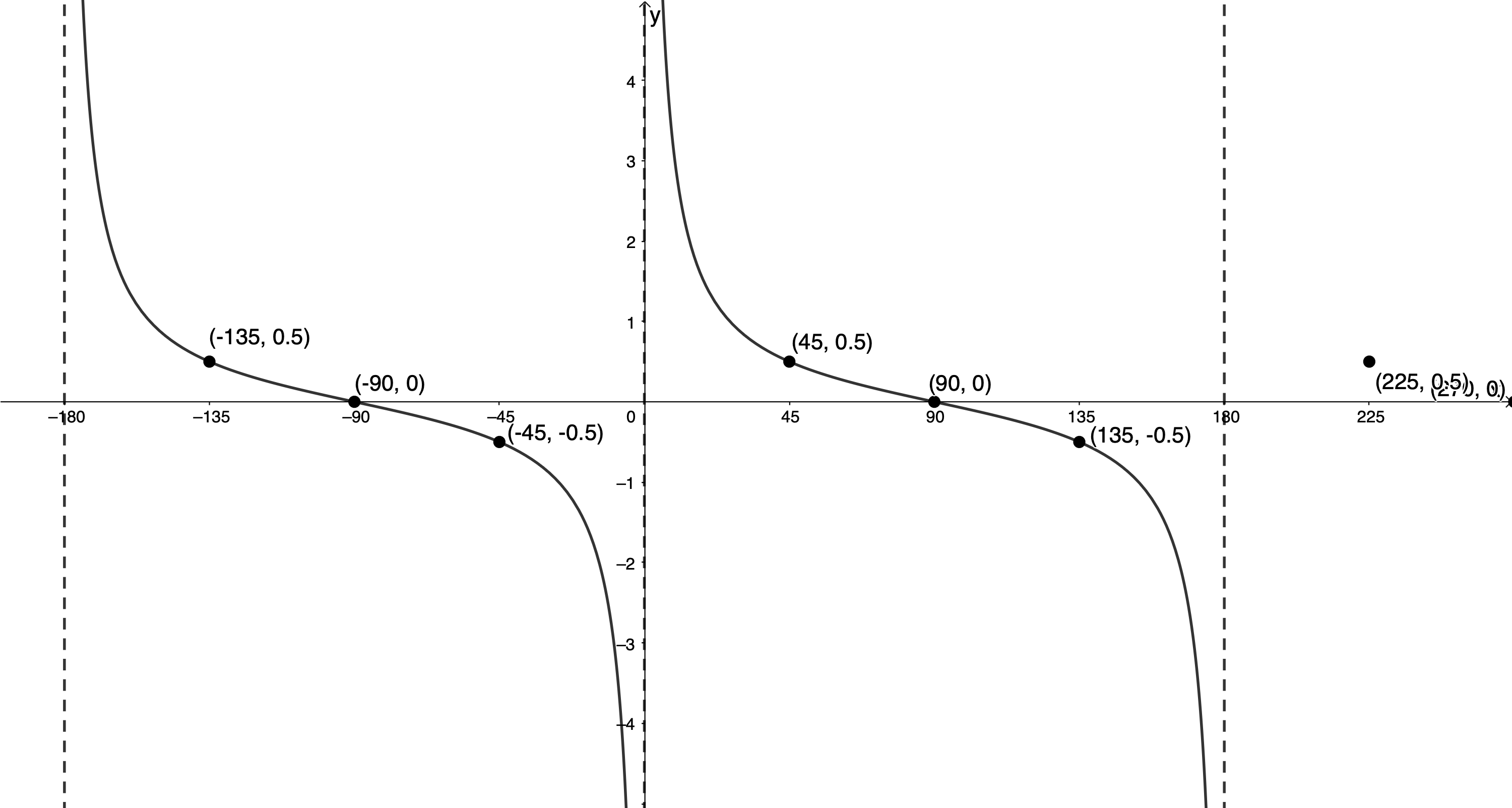
- From the graph below of the form [latex]\scriptsize y=a\tan (x+p)[/latex], determine the values of [latex]\scriptsize a[/latex] and [latex]\scriptsize p[/latex].
The full solutions are at the end of the unit.
Unit 12: Solutions
Exercise 12.1
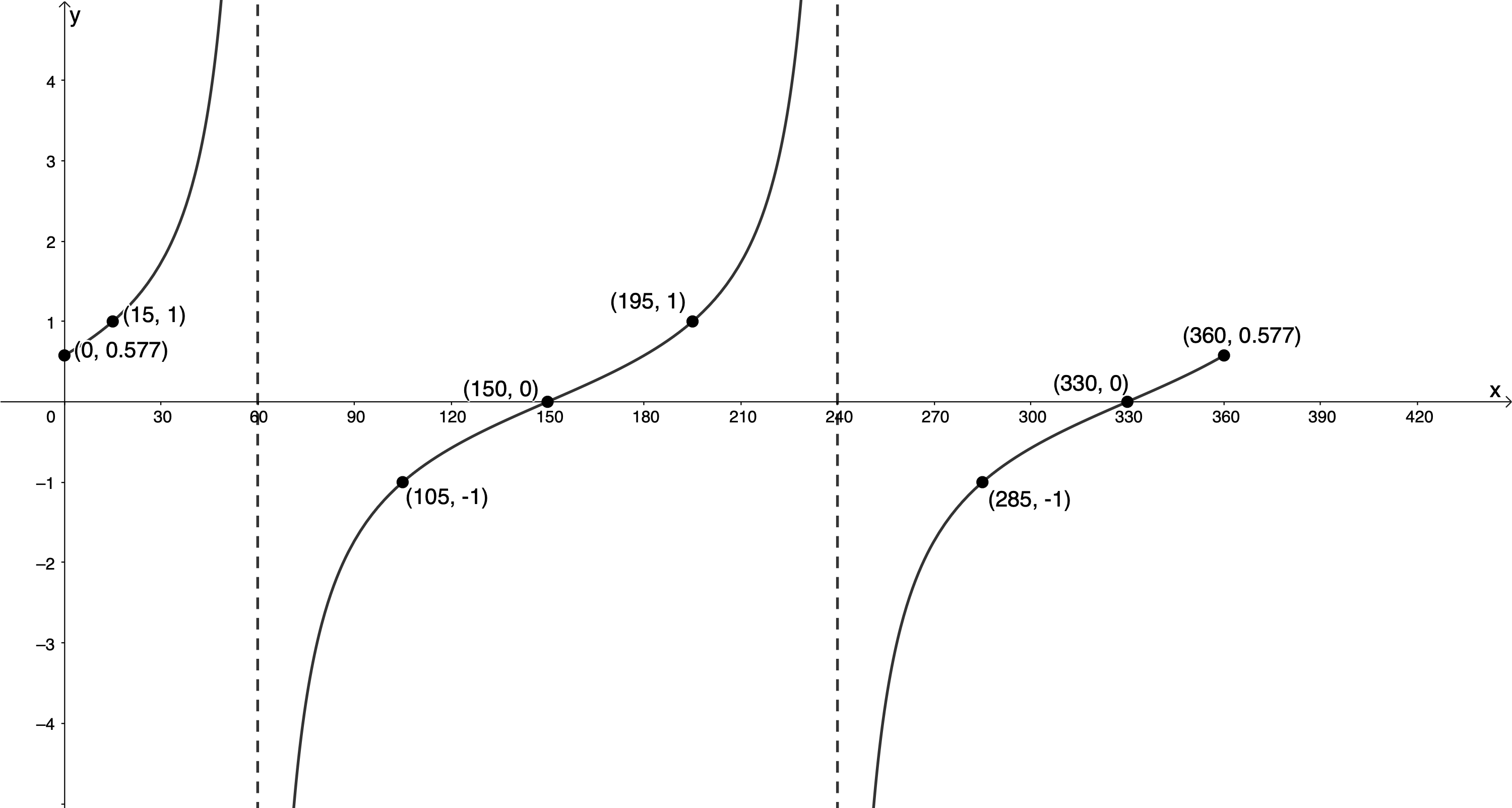
- [latex]\scriptsize f(x)=\tan (x+{{30}^\circ})[/latex] for [latex]\scriptsize {{0}^\circ}\le x\le {{360}^\circ}[/latex]
[latex]\scriptsize p={{30}^\circ}[/latex]. Therefore, the graph will be shifted [latex]\scriptsize {{30}^\circ}[/latex] to the left.[latex]\scriptsize \tan x[/latex] [latex]\scriptsize ({{0}^\circ},0)[/latex] [latex]\scriptsize ({{45}^\circ},1)[/latex] [latex]\scriptsize x={{90}^\circ}[/latex] asymptote [latex]\scriptsize ({{135}^\circ},-1)[/latex] [latex]\scriptsize ({{180}^\circ},0)[/latex] [latex]\scriptsize \tan (x+{{30}^\circ})[/latex] [latex]\scriptsize (-{{30}^\circ},0)[/latex] [latex]\scriptsize ({{15}^\circ},1)[/latex] [latex]\scriptsize x={{60}^\circ}[/latex] asymptote [latex]\scriptsize ({{105}^\circ},-1)[/latex] [latex]\scriptsize ({{150}^\circ},0)[/latex] y-intercept (let [latex]\scriptsize x=0[/latex]):
[latex]\scriptsize \begin{align*}f(0) & =\tan ({{0}^\circ}+{{30}^\circ})\\\therefore f(0) & =\displaystyle \frac{1}{{\sqrt{3}}}=0.577\end{align*}[/latex]
.
Because the period of the function is [latex]\scriptsize {{180}^\circ}[/latex] we know that the function value at [latex]\scriptsize {{180}^\circ}[/latex] will also be [latex]\scriptsize 0.577[/latex].
.
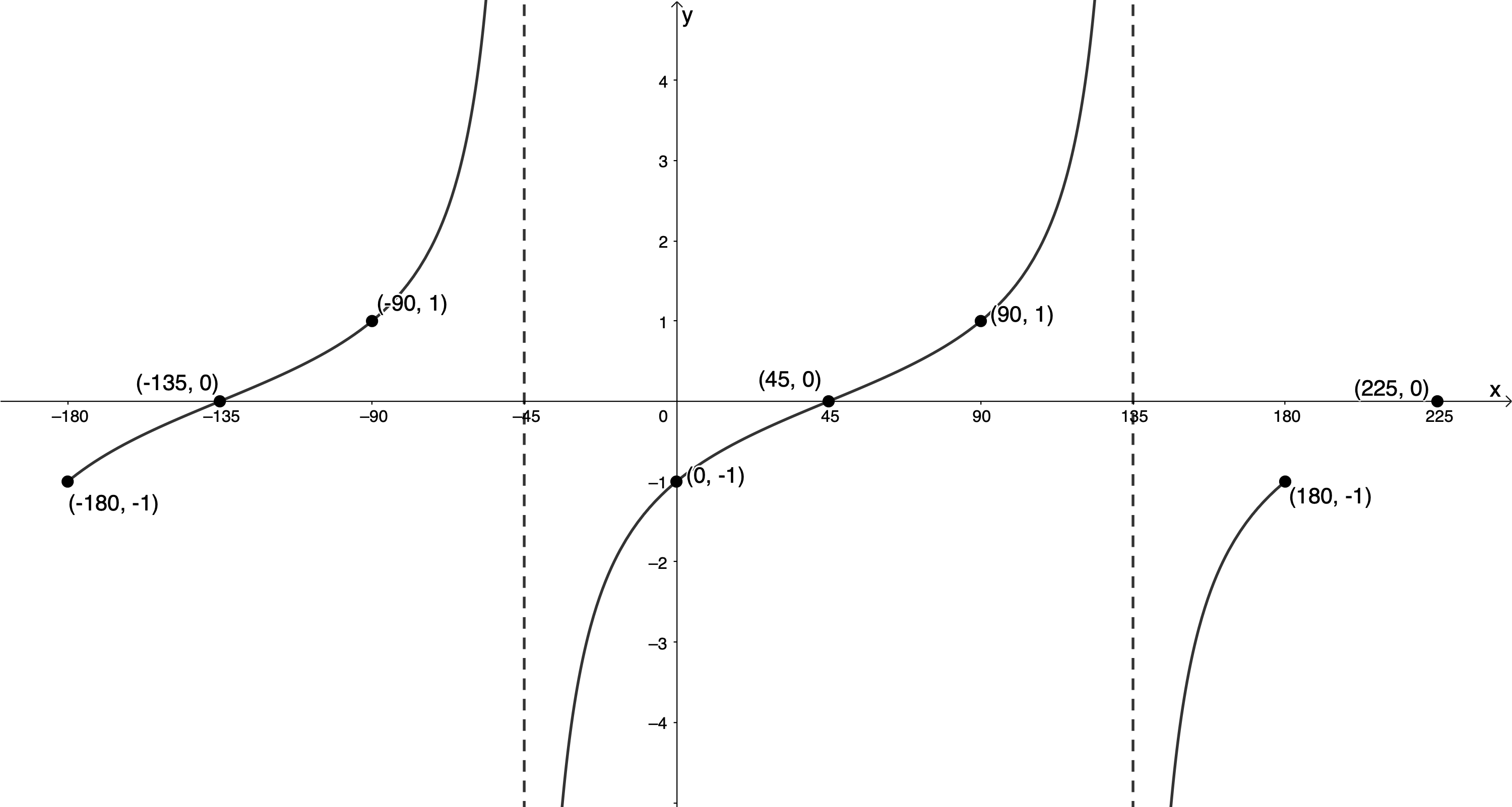
- [latex]\scriptsize g(x)=\tan (x-{{45}^\circ})[/latex] for [latex]\scriptsize -{{180}^\circ}\le x\le {{180}^\circ}[/latex]
[latex]\scriptsize p=-{{45}^\circ}[/latex]. Therefore, the graph will be shifted [latex]\scriptsize {{45}^\circ}[/latex] to the right.[latex]\scriptsize \tan x[/latex] [latex]\scriptsize ({{0}^\circ},0)[/latex] [latex]\scriptsize ({{45}^\circ},1)[/latex] [latex]\scriptsize x={{90}^\circ}[/latex] asymptote [latex]\scriptsize ({{135}^\circ},-1)[/latex] [latex]\scriptsize ({{180}^\circ},0)[/latex] [latex]\scriptsize \tan (x-{{45}^\circ})[/latex] [latex]\scriptsize ({{45}^\circ},0)[/latex] [latex]\scriptsize ({{90}^\circ},1)[/latex] [latex]\scriptsize x={{135}^\circ}[/latex] asymptote [latex]\scriptsize ({{180}^\circ},-1)[/latex] [latex]\scriptsize ({{225}^\circ},0)[/latex] y-intercept (let [latex]\scriptsize x=0[/latex]):
[latex]\scriptsize \begin{align*}g(0) & =\tan ({{0}^\circ}-{{45}^\circ})\\\therefore g(0) & =-1\end{align*}[/latex]
.
Because the period of the function is [latex]\scriptsize {{180}^\circ}[/latex] we know that the function values at [latex]\scriptsize -{{180}^\circ}[/latex] and [latex]\scriptsize {{180}^\circ}[/latex] will also be [latex]\scriptsize 1[/latex].
.
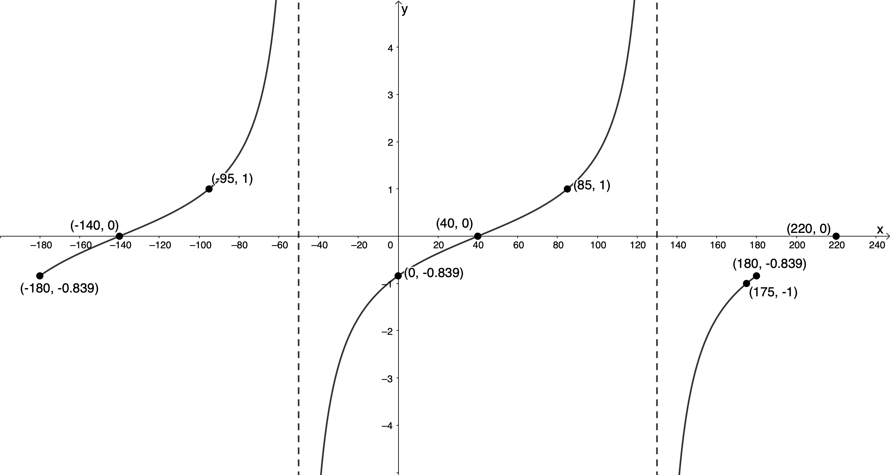
- [latex]\scriptsize h(x)=\tan (x-{{40}^\circ})[/latex] for [latex]\scriptsize -{{180}^\circ}\le x\le {{180}^\circ}[/latex]
[latex]\scriptsize p=-{{40}^\circ}[/latex]. Therefore, the graph will be shifted [latex]\scriptsize {{40}^\circ}[/latex] to the right.[latex]\scriptsize \tan x[/latex] [latex]\scriptsize ({{0}^\circ},0)[/latex] [latex]\scriptsize ({{45}^\circ},1)[/latex] [latex]\scriptsize x={{90}^\circ}[/latex] asymptote [latex]\scriptsize ({{135}^\circ},-1)[/latex] [latex]\scriptsize ({{180}^\circ},0)[/latex] [latex]\scriptsize \tan (x-{{40}^\circ})[/latex] [latex]\scriptsize ({{40}^\circ},0)[/latex] [latex]\scriptsize ({{85}^\circ},1)[/latex] [latex]\scriptsize x={{130}^\circ}[/latex] asymptote [latex]\scriptsize ({{175}^\circ},-1)[/latex] [latex]\scriptsize ({{220}^\circ},0)[/latex] y-intercept (let [latex]\scriptsize x=0[/latex]):
[latex]\scriptsize \begin{align*}h(0) & =\tan ({{0}^\circ}-{{40}^\circ})\\\therefore h(0) & =-0.839\end{align*}[/latex]
.
Because the period of the function is [latex]\scriptsize {{180}^\circ}[/latex] we know that the function values at [latex]\scriptsize -{{180}^\circ}[/latex] and [latex]\scriptsize {{180}^\circ}[/latex] will also be [latex]\scriptsize -0.839[/latex].
.
Exercise 12.2
- [latex]\scriptsize y=-2\tan (x+{{45}^\circ})[/latex] for [latex]\scriptsize {{0}^\circ}\le x\le {{180}^\circ}[/latex]
[latex]\scriptsize a=-2[/latex]. Therefore, the graph be reflected about the x-axis.
[latex]\scriptsize p={{45}^\circ}[/latex]. Therefore, the graph will be shifted [latex]\scriptsize {{45}^\circ}[/latex] to the left.[latex]\scriptsize \tan x[/latex] [latex]\scriptsize ({{0}^\circ},0)[/latex] [latex]\scriptsize ({{45}^\circ},1)[/latex] [latex]\scriptsize x={{90}^\circ}[/latex] asymptote [latex]\scriptsize ({{135}^\circ},-1)[/latex] [latex]\scriptsize ({{180}^\circ},0)[/latex] [latex]\scriptsize -2\tan (x+{{45}^\circ})[/latex] [latex]\scriptsize (-{{45}^\circ},0)[/latex] [latex]\scriptsize ({{0}^\circ},-2)[/latex] [latex]\scriptsize x={{45}^\circ}[/latex] asymptote [latex]\scriptsize ({{90}^\circ},2)[/latex] [latex]\scriptsize ({{135}^\circ},0)[/latex] y-intercept (let [latex]\scriptsize x=0[/latex]):
[latex]\scriptsize \begin{align*}y & =-2\tan ({{0}^\circ}+{{45}^\circ})\\\therefore y & =-2\times 1\\&=-2\end{align*}[/latex]
.
Because the period of the function is [latex]\scriptsize {{180}^\circ}[/latex] we know that the function value at [latex]\scriptsize {{180}^\circ}[/latex] will also be [latex]\scriptsize -2[/latex].
.
.
y-intercept: [latex]\scriptsize ({{0}^\circ},-2)[/latex]
x-intercepts: [latex]\scriptsize ({{135}^\circ},0)[/latex]
Domain: [latex]\scriptsize \{x|x\in \mathbb{R},\text{ }{{0}^\circ}\le x\le {{180}^\circ};x\ne 45{}^\circ \}[/latex]
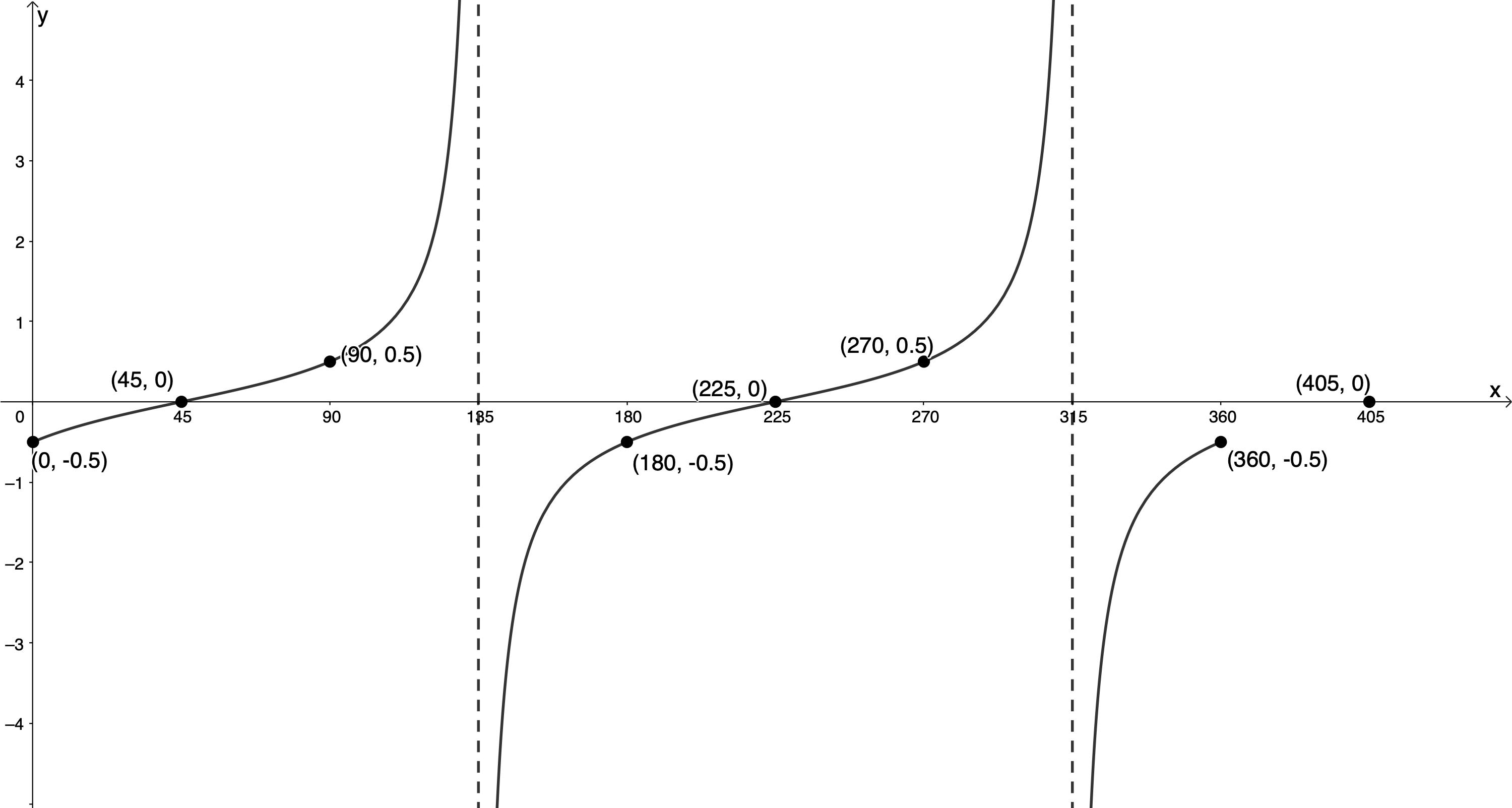
Range: [latex]\scriptsize \{y|y\in \mathbb{R}\}\text{ }[/latex] - [latex]\scriptsize 2y=\tan (x-{{45}^\circ})[/latex] for [latex]\scriptsize {{0}^\circ}\le x\le {{360}^\circ}[/latex]
[latex]\scriptsize \begin{align*}2y & =\tan (x-{{45}^\circ})\\\therefore y & =\displaystyle \frac{1}{2}\tan (x-{{45}^\circ})\end{align*}[/latex]
[latex]\scriptsize a=\displaystyle \frac{1}{2}[/latex]. The graph will not be reflected about the x-axis.
[latex]\scriptsize p=-{{45}^\circ}[/latex]. Therefore, the graph will be shifted [latex]\scriptsize {{45}^\circ}[/latex] to the right.[latex]\scriptsize \tan x[/latex] [latex]\scriptsize ({{0}^\circ},0)[/latex] [latex]\scriptsize ({{45}^\circ},1)[/latex] [latex]\scriptsize x={{90}^\circ}[/latex] asymptote [latex]\scriptsize ({{135}^\circ},-1)[/latex] [latex]\scriptsize ({{180}^\circ},0)[/latex] [latex]\scriptsize \displaystyle \frac{1}{2}\tan (x-{{45}^\circ})[/latex] [latex]\scriptsize ({{45}^\circ},0)[/latex] [latex]\scriptsize ({{90}^\circ},\displaystyle \frac{1}{2})[/latex] [latex]\scriptsize x={{135}^\circ}[/latex] asymptote [latex]\scriptsize ({{180}^\circ},-\displaystyle \frac{1}{2})[/latex] [latex]\scriptsize ({{225}^\circ},0)[/latex] y-intercept (let [latex]\scriptsize x=0[/latex]):
[latex]\scriptsize \begin{align*}y & =\displaystyle \frac{1}{2}\tan ({{0}^\circ}-{{45}^\circ})\\\therefore y & =\displaystyle \frac{1}{2}\times (-1)=-\displaystyle \frac{1}{2}\end{align*}[/latex]
.
Because the period of the function is [latex]\scriptsize {{180}^\circ}[/latex] we know that the function value at [latex]\scriptsize {{180}^\circ}[/latex] and [latex]\scriptsize {{360}^\circ}[/latex] will also be [latex]\scriptsize -\displaystyle \frac{1}{2}[/latex].
.
.
y-intercept: [latex]\scriptsize ({{0}^\circ},-\displaystyle \frac{1}{2})[/latex]
x-intercepts: [latex]\scriptsize ({{45}^\circ},0)[/latex], [latex]\scriptsize ({{225}^\circ},0)[/latex]
Domain: [latex]\scriptsize \{x|x\in \mathbb{R},\text{ }{{0}^\circ}\le x\le {{360}^\circ};x\ne 135{}^\circ \text{ or }315{}^\circ \}[/latex]
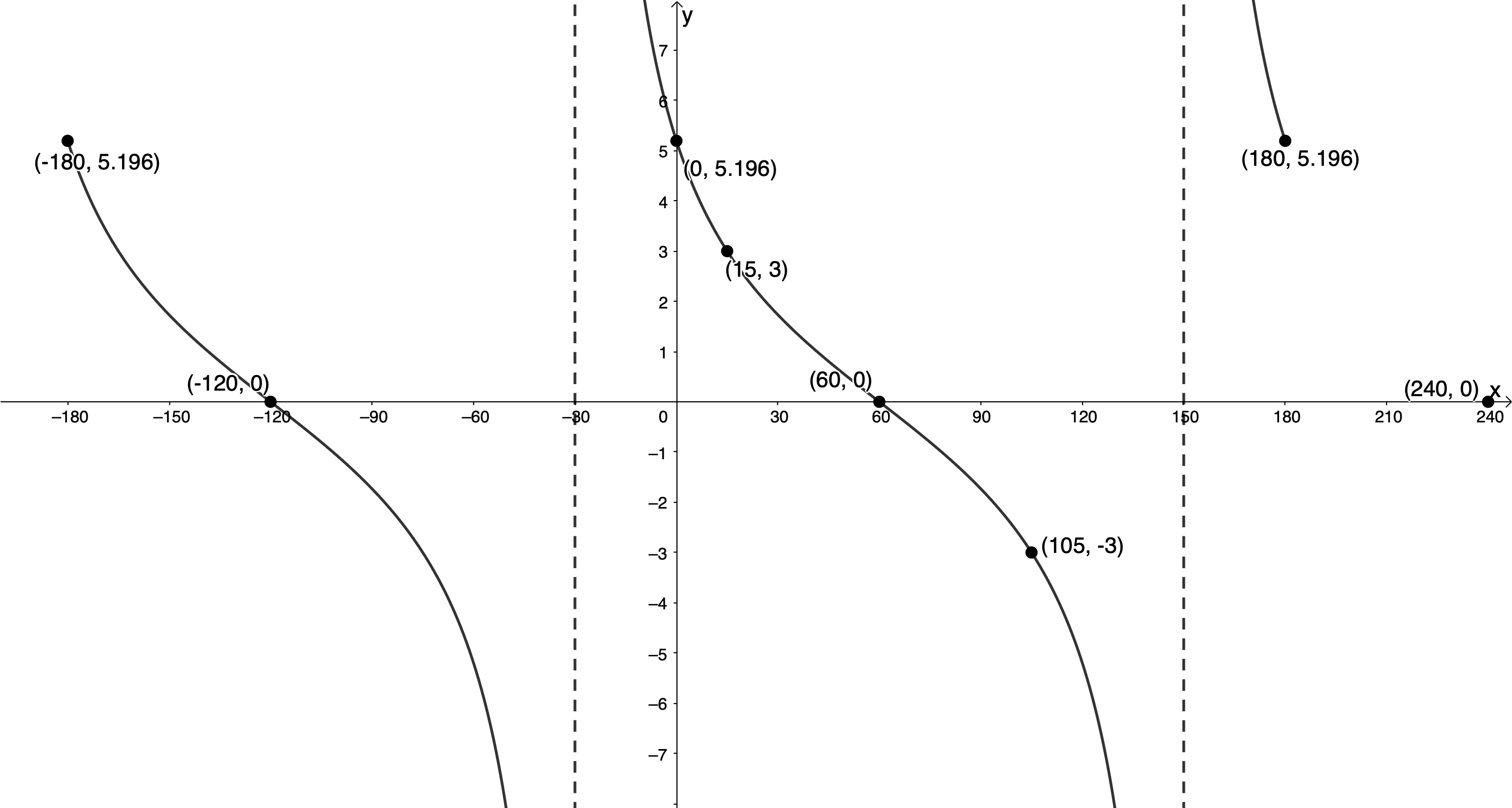
Range: [latex]\scriptsize \{y|y\in \mathbb{R}\}\text{ }[/latex] - [latex]\scriptsize \displaystyle \frac{1}{3}y=\tan ({{60}^\circ}-x)[/latex] for [latex]\scriptsize -{{180}^\circ}\le x\le {{180}^\circ}[/latex]
[latex]\scriptsize \begin{align*}\displaystyle \frac{1}{3}y & =\tan ({{60}^\circ}-x)\\\therefore y & =3\tan ({{60}^\circ}-x)\\&=3\tan (-x+{{60}^\circ})\\&=3\tan \left( {-\left( {x-{{{60}}^\circ}} \right)} \right)\\&=-3\tan (x-{{60}^\circ})\end{align*}[/latex]
[latex]\scriptsize a=-3[/latex]. Therefore, the graph will be reflected about the x-axis.
[latex]\scriptsize p=-{{60}^\circ}[/latex]. Therefore, the graph will be shifted [latex]\scriptsize {{60}^\circ}[/latex] to the right.[latex]\scriptsize \tan x[/latex] [latex]\scriptsize ({{0}^\circ},0)[/latex] [latex]\scriptsize ({{45}^\circ},1)[/latex] [latex]\scriptsize x={{90}^\circ}[/latex] asymptote [latex]\scriptsize ({{135}^\circ},-1)[/latex] [latex]\scriptsize ({{180}^\circ},0)[/latex] [latex]\scriptsize -3\tan (x-{{60}^\circ})[/latex] [latex]\scriptsize ({{60}^\circ},0)[/latex] [latex]\scriptsize ({{105}^\circ},-3)[/latex] [latex]\scriptsize x={{150}^\circ}[/latex] asymptote [latex]\scriptsize ({{195}^\circ},3)[/latex] [latex]\scriptsize ({{240}^\circ},0)[/latex] y-intercept (let [latex]\scriptsize x=0[/latex]):
[latex]\scriptsize \begin{align*}y & =-3\tan ({{0}^\circ}-{{60}^\circ})\text{ }\\\therefore y & =-3\times -\displaystyle \frac{{\sqrt{3}}}{1}=3\sqrt{3}\\&=5.196\end{align*}[/latex]
.
Because the period of the function is [latex]\scriptsize {{180}^\circ}[/latex] we know that the function values at [latex]\scriptsize -{{180}^\circ}[/latex] and [latex]\scriptsize {{180}^\circ}[/latex] will also be [latex]\scriptsize 5.196[/latex].
.
.
y-intercept: [latex]\scriptsize ({{0}^\circ},5.196)[/latex] or [latex]\scriptsize ({{0}^\circ},3\sqrt{3})[/latex]
x-intercepts: [latex]\scriptsize (-{{120}^\circ},0)[/latex], [latex]\scriptsize ({{60}^\circ},0)[/latex]
Domain: [latex]\scriptsize \{x|x\in \mathbb{R},\text{ }-{{180}^\circ}\le x\le {{180}^\circ};x\ne -30{}^\circ ;x\ne 150{}^\circ \}[/latex]
Range: [latex]\scriptsize \{y|y\in \mathbb{R}\}\text{ }[/latex]
Exercise 12.3
- The asymptote is at [latex]\scriptsize x={{105}^\circ}=({{90}^\circ}+{{15}^\circ})[/latex]. Therefore, the graph has been shifted [latex]\scriptsize {{15}^\circ}[/latex] to the right and [latex]\scriptsize p=-{{15}^\circ}[/latex].
[latex]\scriptsize ({{45}^\circ},1)[/latex] has been transformed to [latex]\scriptsize ({{60}^\circ},2.5)[/latex]. Therefore, [latex]\scriptsize a=2.5[/latex].
[latex]\scriptsize y=2.5\tan (x-{{15}^\circ})[/latex] - Domain: [latex]\scriptsize \{x|x\in \mathbb{R},\text{ }{{0}^\circ}\le x\le {{360}^\circ};x\ne 105{}^\circ ,285{}^\circ \}[/latex]
Range: [latex]\scriptsize \{y|y\in \mathbb{R}\}\text{ }[/latex]
Unit 12: Assessment
- .
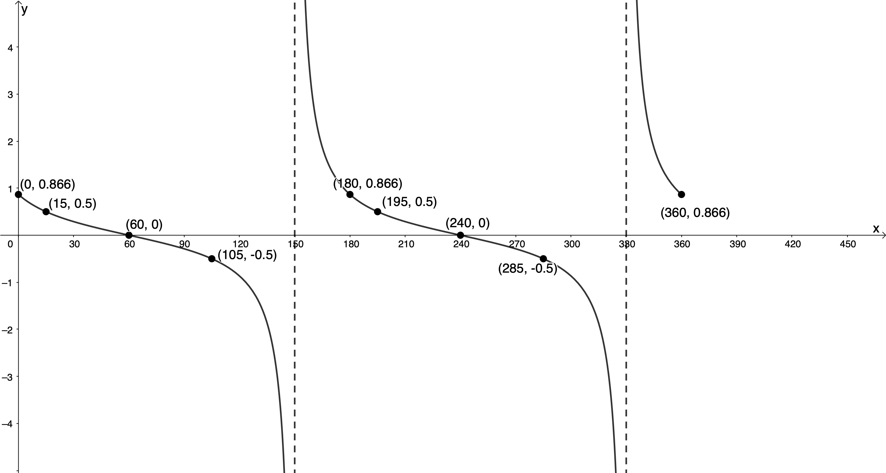
- [latex]\scriptsize 2y=-\tan \left( {x-{{{60}}^\circ}} \right)[/latex] for [latex]\scriptsize {{0}^\circ}\le x\le {{360}^\circ}[/latex]
[latex]\scriptsize \begin{align*}2y & =-\tan (x-{{60}^\circ})\\\therefore y & =-\displaystyle \frac{1}{2}\tan (x-{{60}^\circ})\end{align*}[/latex]
[latex]\scriptsize a=-\displaystyle \frac{1}{2}[/latex]. Therefore, the graph will be reflected about the x-axis.
[latex]\scriptsize p=-{{60}^\circ}[/latex]. Therefore, the graph will be shifted [latex]\scriptsize {{60}^\circ}[/latex] to the right.[latex]\scriptsize \tan x[/latex] [latex]\scriptsize ({{0}^\circ},0)[/latex] [latex]\scriptsize ({{45}^\circ},1)[/latex] [latex]\scriptsize x={{90}^\circ}[/latex] asymptote [latex]\scriptsize ({{135}^\circ},-1)[/latex] [latex]\scriptsize ({{180}^\circ},0)[/latex] [latex]\scriptsize -\displaystyle \frac{1}{2}\tan (x-{{60}^\circ})[/latex] [latex]\scriptsize ({{60}^\circ},0)[/latex] [latex]\scriptsize ({{105}^\circ},-\displaystyle \frac{1}{2})[/latex] [latex]\scriptsize x={{150}^\circ}[/latex] asymptote [latex]\scriptsize ({{195}^\circ},\displaystyle \frac{1}{2})[/latex] [latex]\scriptsize ({{240}^\circ},0)[/latex] y-intercept (let [latex]\scriptsize x=0[/latex]):
[latex]\scriptsize \begin{align*}y & =-\displaystyle \frac{1}{2}\tan ({{0}^\circ}-{{60}^\circ})\\\therefore y & =-\displaystyle \frac{1}{2}\times -\displaystyle \frac{{\sqrt{3}}}{1}=\displaystyle \frac{{\sqrt{3}}}{2}=0.866\end{align*}[/latex]
.
Because the period of the function is [latex]\scriptsize {{180}^\circ}[/latex] we know that the function value at [latex]\scriptsize {{180}^\circ}[/latex] and [latex]\scriptsize {{360}^\circ}[/latex] will also be [latex]\scriptsize 0.866[/latex].
.
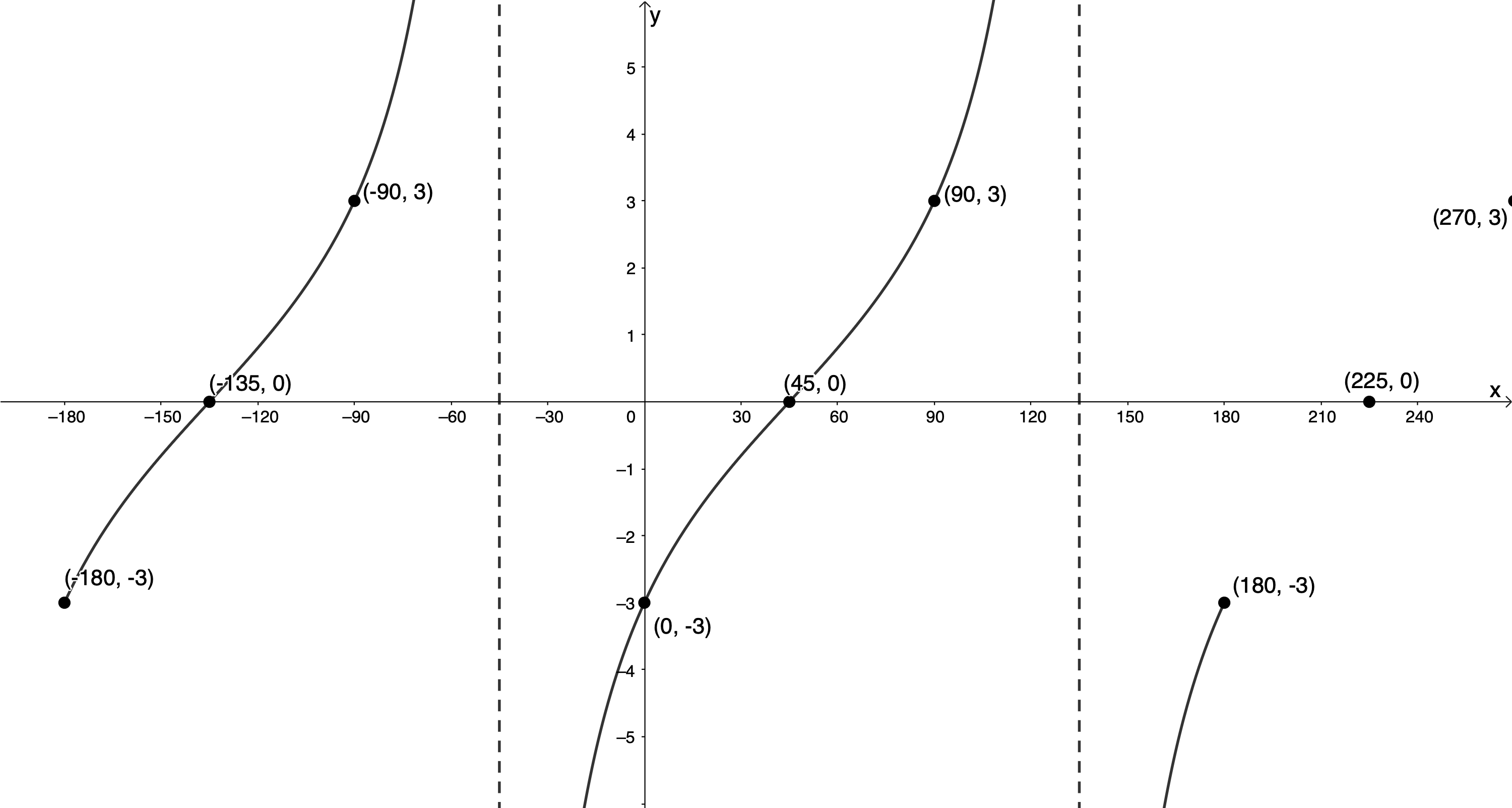
- [latex]\scriptsize g(x)=-3\tan ({{45}^\circ}-x)[/latex] for [latex]\scriptsize -{{180}^\circ}\le x\le {{180}^\circ}[/latex]
[latex]\scriptsize \begin{align*}g(x) & =-3\tan ({{45}^\circ}-x)\\&=-3\tan (-x+{{45}^\circ})\\&=-3\tan \left( {-\left( {x-{{{45}}^\circ}} \right)} \right)\\&=3\tan (x-{{45}^\circ})\end{align*}[/latex]
[latex]\scriptsize a=3[/latex]. Therefore, the graph will not be reflected about the x-axis.
[latex]\scriptsize \displaystyle p=-{{45}^\circ}[/latex]. Therefore, the graph will be shifted [latex]\scriptsize {{45}^\circ}[/latex] to the right.[latex]\scriptsize \tan x[/latex] [latex]\scriptsize ({{0}^\circ},0)[/latex] [latex]\scriptsize ({{45}^\circ},1)[/latex] [latex]\scriptsize x={{90}^\circ}[/latex] asymptote [latex]\scriptsize ({{135}^\circ},-1)[/latex] [latex]\scriptsize ({{180}^\circ},0)[/latex] [latex]\scriptsize 3\tan (x-{{45}^\circ})[/latex] [latex]\scriptsize ({{45}^\circ},0)[/latex] [latex]\scriptsize ({{90}^\circ},3)[/latex] [latex]\scriptsize x={{135}^\circ}[/latex] asymptote [latex]\scriptsize ({{180}^\circ},-3)[/latex] [latex]\scriptsize ({{225}^\circ},0)[/latex] y-intercept (let [latex]\scriptsize x=0[/latex]):
[latex]\scriptsize \begin{align*}g(0)&=3\tan ({{0}^\circ}-{{45}^\circ})\\ \therefore y&=3 \times -1=-3\end{align*}[/latex]
.
Because the period of the function is [latex]\scriptsize {{180}^\circ}[/latex] we know that the function values at [latex]\scriptsize -{{180}^\circ}[/latex] and [latex]\scriptsize {{180}^\circ}[/latex] will also be [latex]\scriptsize -3[/latex].
.
- [latex]\scriptsize 2y=-\tan \left( {x-{{{60}}^\circ}} \right)[/latex] for [latex]\scriptsize {{0}^\circ}\le x\le {{360}^\circ}[/latex]
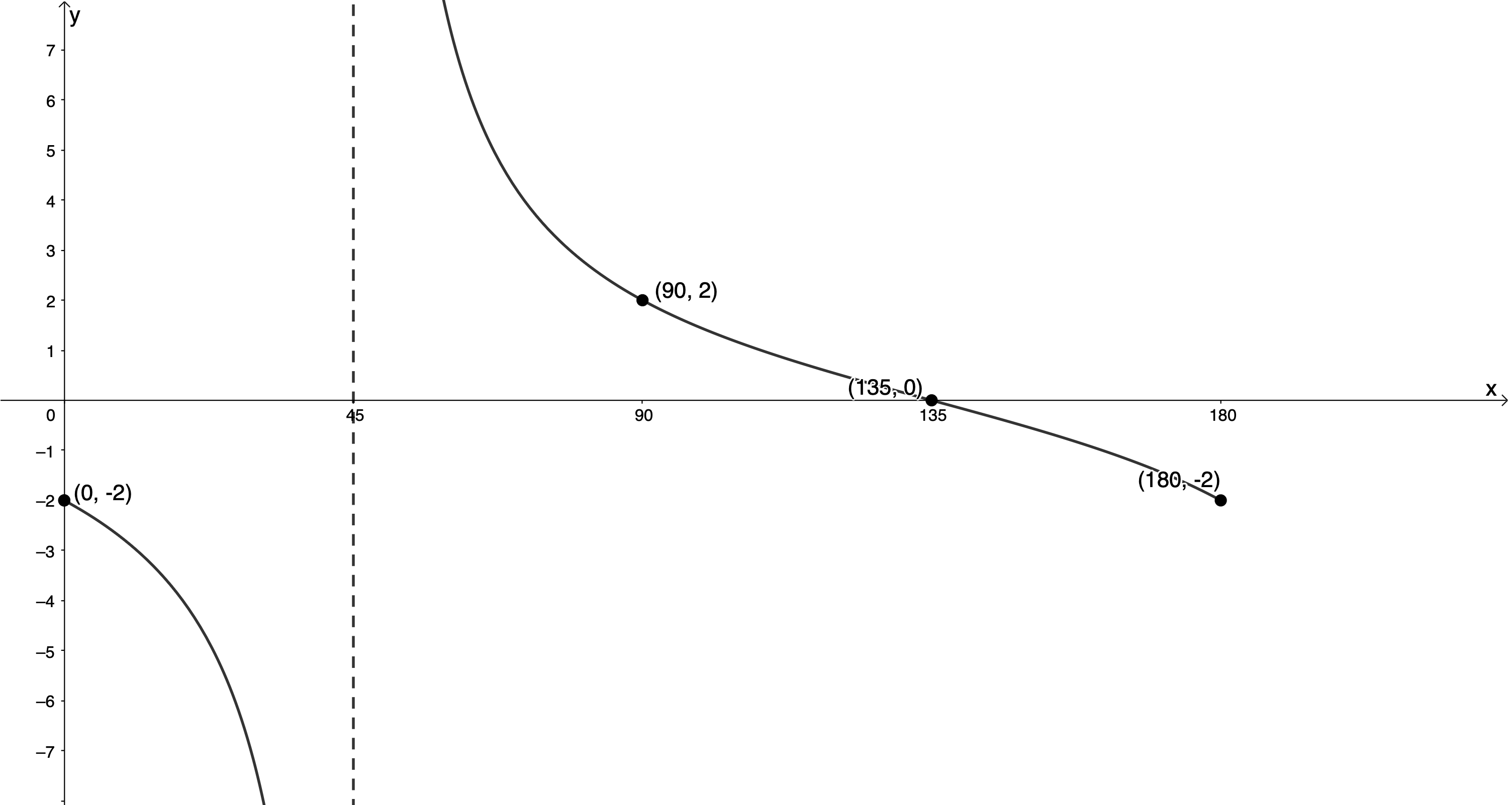
- The function is of the form [latex]\scriptsize y=a\tan (x+p)[/latex]. The asymptote [latex]\scriptsize x={{90}^\circ}[/latex] is now [latex]\scriptsize x={{180}^\circ}[/latex]. Therefore, the graph has been shifted [latex]\scriptsize {{90}^\circ}[/latex] to the right.
.
The function decreases to negative infinity when approaching the asymptote from the left. This means that the function has been reflected about the x-axis and [latex]\scriptsize a \lt 0[/latex].
.
Also, the ‘anchor point’ that was at [latex]\scriptsize ({{45}^\circ},1)[/latex] is now at [latex]\scriptsize ({{135}^\circ},-0.5)[/latex]. Therefore, [latex]\scriptsize a=-\displaystyle \frac{1}{2}[/latex] and the function is [latex]\scriptsize y=-\displaystyle \frac{1}{2}\tan (x-{{90}^\circ})[/latex].
.
However, we can also say that the asymptote [latex]\scriptsize x={{270}^\circ}[/latex] is now [latex]\scriptsize x={{180}^\circ}[/latex] and therefore, the graph has been shifted [latex]\scriptsize {{90}^\circ}[/latex] to the left. Hence [latex]\scriptsize y=-\displaystyle \frac{1}{2}\tan (x+{{90}^\circ})[/latex], which is another possible equation. This means that [latex]\scriptsize \tan (x+{{90}^\circ})=\tan (x-{{90}^\circ})[/latex].
.
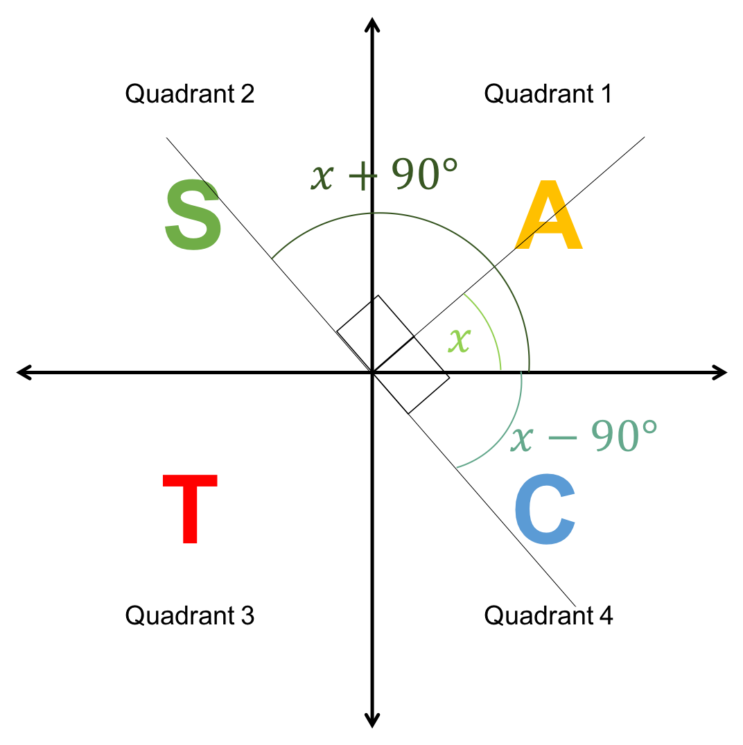
If we assume [latex]\scriptsize {{0}^\circ} \lt x \lt {{90}^\circ}[/latex], we can see why this is the case by looking at the CAST diagram. Tangent is negative in the second and fourth quadrants and [latex]\scriptsize x-{{90}^\circ}[/latex] and [latex]\scriptsize x+{{90}^\circ}[/latex] are the same size angles.
.
Media Attributions
- takenote © DHET is licensed under a CC BY (Attribution) license
- example12.1 © Geogebra is licensed under a CC BY-SA (Attribution ShareAlike) license
- example12.2 © Geogebra is licensed under a CC BY-SA (Attribution ShareAlike) license
- example12.3 © Geogebra is licensed under a CC BY-SA (Attribution ShareAlike) license
- example12.4 © Geogebra is licensed under a CC BY-SA (Attribution ShareAlike) license
- example12.5 © Geogebra is licensed under a CC BY-SA (Attribution ShareAlike) license
- exercise12.3 © Geogebra is licensed under a CC BY-SA (Attribution ShareAlike) license
- assessmentQ2 © Geogebra is licensed under a CC BY-SA (Attribution ShareAlike) license
- exercise12.1A1 © Geogebra is licensed under a CC BY-SA (Attribution ShareAlike) license
- exercise12.1A2 © Geogebra is licensed under a CC BY-SA (Attribution ShareAlike) license
- exercise12.1A3 © Geogebra is licensed under a CC BY-SA (Attribution ShareAlike) license
- exercise12.2A1 © Geogebra is licensed under a CC BY-SA (Attribution ShareAlike) license
- exercise12.2A2 © Geogebra is licensed under a CC BY-SA (Attribution ShareAlike) license
- exercise12.2A3 © Geogebra is licensed under a CC BY-SA (Attribution ShareAlike) license
- assessmentA1a © Geogebra is licensed under a CC BY-SA (Attribution ShareAlike) license
- assessmentA1b © Geogebra is licensed under a CC BY-SA (Attribution ShareAlike) license
- CAST © DHET is licensed under a CC BY (Attribution) license
