Functions and algebra: Use Mathematical models to investigate linear programming problems
Unit 1: Linear programming
Dylan Busa
Unit outcomes
By the end of this unit you will be able to:
- Sketch given constraints.
- Find the feasible region and objective function.
- Use a boundary search to find the vertices of the feasible region.
- Optimise the objective function.
What you should know
Before you start this unit, make sure you can:
- Simplify algebraic expressions including those with fractions. Refer to level 2 subject outcome 2.2 unit 1 and unit 3 if you need help with this.
- Solve linear equations. Refer to level 2 subject outcomes 2.3 unit 1 if you need help with this.
- Solve linear inequalities. Refer to level 3 subject outcome 2.3 unit 3 if you need help with this.
- Sketch graphs of linear functions. Refer to level 2 subject outcome 2.1 unit 1 if you need help with this.
Introduction
Qhubeka is a wonderful organisation that donates bicycles to children in rural areas to make things such as getting to and from school easier and quicker.
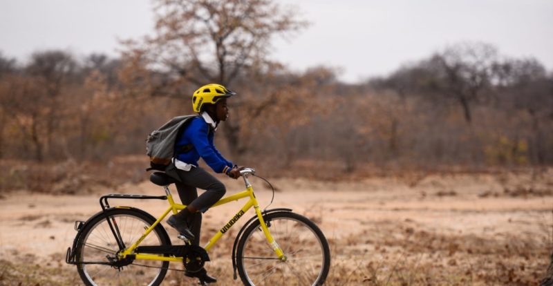
Qhubeka makes all the bicycles it donates, thereby also creating employment. Suppose it makes two types of bicycles – the Buffalo and the Cheetah. The Buffalo is rugged and designed for areas where the roads aren’t so good. The Cheetah is designed for areas where there are at least basic roads.
Now suppose that each day Qhubeka can produce at most seven Buffalos and six Cheetahs. It takes three technicians to build a Buffalo and two technicians to build a Cheetah. There is a total of [latex]\scriptsize 18[/latex] technicians at the organisation.
Each Buffalo costs [latex]\scriptsize \text{R2}\ 400[/latex] to make and each Cheetah costs [latex]\scriptsize \text{R1}\ 200[/latex] to make. If every bicycle that Qhubeka makes is needed by a child, how many of each type should Qhubeka make in order to minimise costs?
This is an example of an optimisation problem. There are several constraints that all need to be taken into account to find an optimal solution, in this case the lowest cost.
Another example of an optimisation problem would be a farmer working out how much of two different crops to plant, with different input costs and different market values, in order to maximise his profit. In all cases, we want to calculate the maximum or minimum in a specific situation.
Solve optimisation problems graphically
The easiest and most efficient way to solve these kinds of optimisation problems is graphically using a technique called linear programming. Linear programming is a graphical modelling technique in which the optimal solution of a linear function is found by applying various other constraints. Linear programming is, therefore, a special case of the broader area of mathematical programming and is most often used to guide decision making in business, engineering, social sciences, and physical sciences.
A detailed worked example of the solution to the problem Qhubeka faces is the best way to demonstrate how linear programming works.
Example 1.1
This is what we know:
- Qhubeka makes two types of bicycles – the Buffalo and the Cheetah.
- Each day Qhubeka can produce at most seven Buffalos and four Cheetahs.
- Each Buffalo needs three technicians to build it.
- Each Cheetah needs two technicians.
- There is a total of [latex]\scriptsize 18[/latex] technicians.
- Each Buffalo costs [latex]\scriptsize \text{R2}\ 400[/latex] to make and each Cheetah costs [latex]\scriptsize \text{R1}\ 200[/latex] to make.
- If every bicycle that Qhubeka makes is needed by a child, how many of each type should Qhubeka make per day in order to minimise costs?
- What is this minimum cost?
Solution
There are five basic steps to using linear programming to solve optimisation problems.
Step 1: Assign variables
In this problem, there are two types of bicycles and we want to find out how many of each kind should be produced. We need to assign a variable to each type of bicycle. You can assign any variables you like but, because we will be sketching linear functions, it is often simplest to just use [latex]\scriptsize x[/latex] and [latex]\scriptsize y[/latex].
Let the number of Buffalo bicycles be [latex]\scriptsize x[/latex].
Let the number of Cheetah bicycles be [latex]\scriptsize y[/latex].
In both cases, the values of [latex]\scriptsize x[/latex] and [latex]\scriptsize y[/latex] are limited to natural numbers. We cannot have a fraction of a bicycle. Therefore [latex]\scriptsize \{x|x\in \mathbb{N}\}\text{ }[/latex] and [latex]\scriptsize \{y|y\in \mathbb{N}\}\text{ }[/latex].
Step 2: Express the constraints
In all cases a set of constraints is given to you. The first constraint we are given is that each day at most seven Buffalo bicycles can be built. Therefore, [latex]\scriptsize x\le 7[/latex].
We are also told that at most four Cheetah bicycles can be built. Therefore, [latex]\scriptsize y\le 4[/latex].
Each Buffalo needs three technicians and each Cheetah needs two technicians. But there are only [latex]\scriptsize 18[/latex] technicians. Therefore, we can say that [latex]\scriptsize 3x+2y\le 18[/latex] where [latex]\scriptsize 3x[/latex] is the total number of technicians needed to build [latex]\scriptsize x[/latex] Buffalos and [latex]\scriptsize 2y[/latex] is the total number of technicians needed to build [latex]\scriptsize y[/latex] Cheetahs.
Step 3: Determine the objective function
The objective function is the linear function we are trying to find a maximum or minimum solution for. In our case, we need to minimise cost. We are told that each Buffalo costs [latex]\scriptsize \text{R2}\ 400[/latex] to make and each Cheetah costs [latex]\scriptsize \text{R1}\ 200[/latex] to make. Therefore, [latex]\scriptsize 2\ 400x+1\ 200y=C[/latex] where [latex]\scriptsize C[/latex] is the total cost of producing [latex]\scriptsize x[/latex] Buffalo bicycles and [latex]\scriptsize y[/latex] Cheetah bicycles.
Step 4: Graph the constraints
It is time to start graphing our constraints so that we can optimise the objective function. Here are our constraints:
- [latex]\scriptsize x\le 7[/latex]
- [latex]\scriptsize y\le 4[/latex]
- [latex]\scriptsize 3x+2y\le 18[/latex]
Let’s start with [latex]\scriptsize x\le 7[/latex]. If we plot the graph of [latex]\scriptsize x=7[/latex] we get a vertical line that cuts the x-axis at [latex]\scriptsize 7[/latex]. But our graph needs to show [latex]\scriptsize x\le 7[/latex]. Therefore, this is not a line but a region (see Figure 2). Remember that [latex]\scriptsize x\in \mathbb{N}\text{ }[/latex] so we are only including natural numbers between zero and seven.
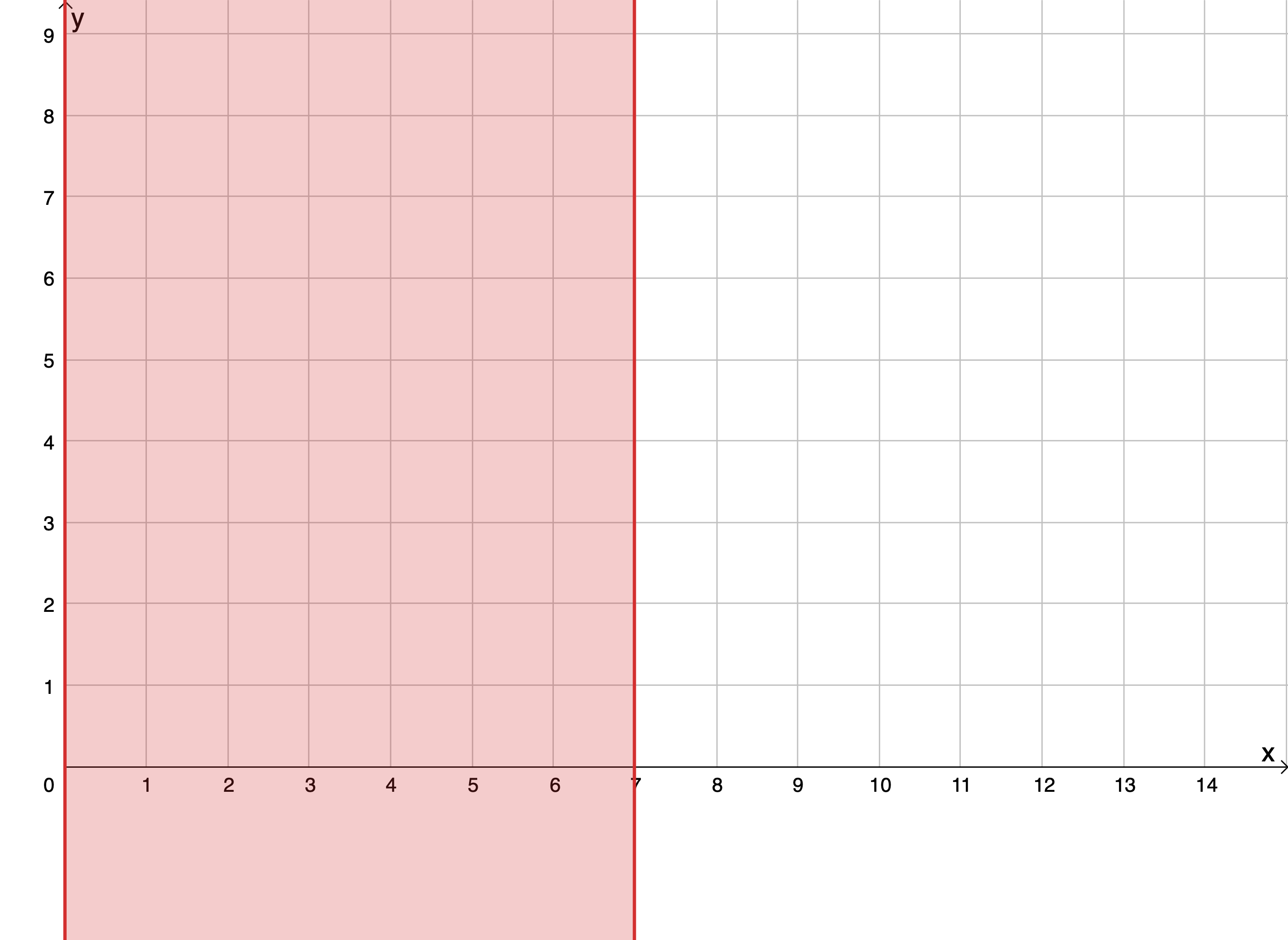
Next, we graph the next constraint, [latex]\scriptsize y\le 4[/latex] (see Figure 3). Again, [latex]\scriptsize y\in \mathbb{N}\text{ }[/latex] so we are only including natural numbers between zero and four.
The overlapping region is what we are interested in because this represents all the values for [latex]\scriptsize x[/latex] and [latex]\scriptsize y[/latex] that would satisfy both constraints at the same time.
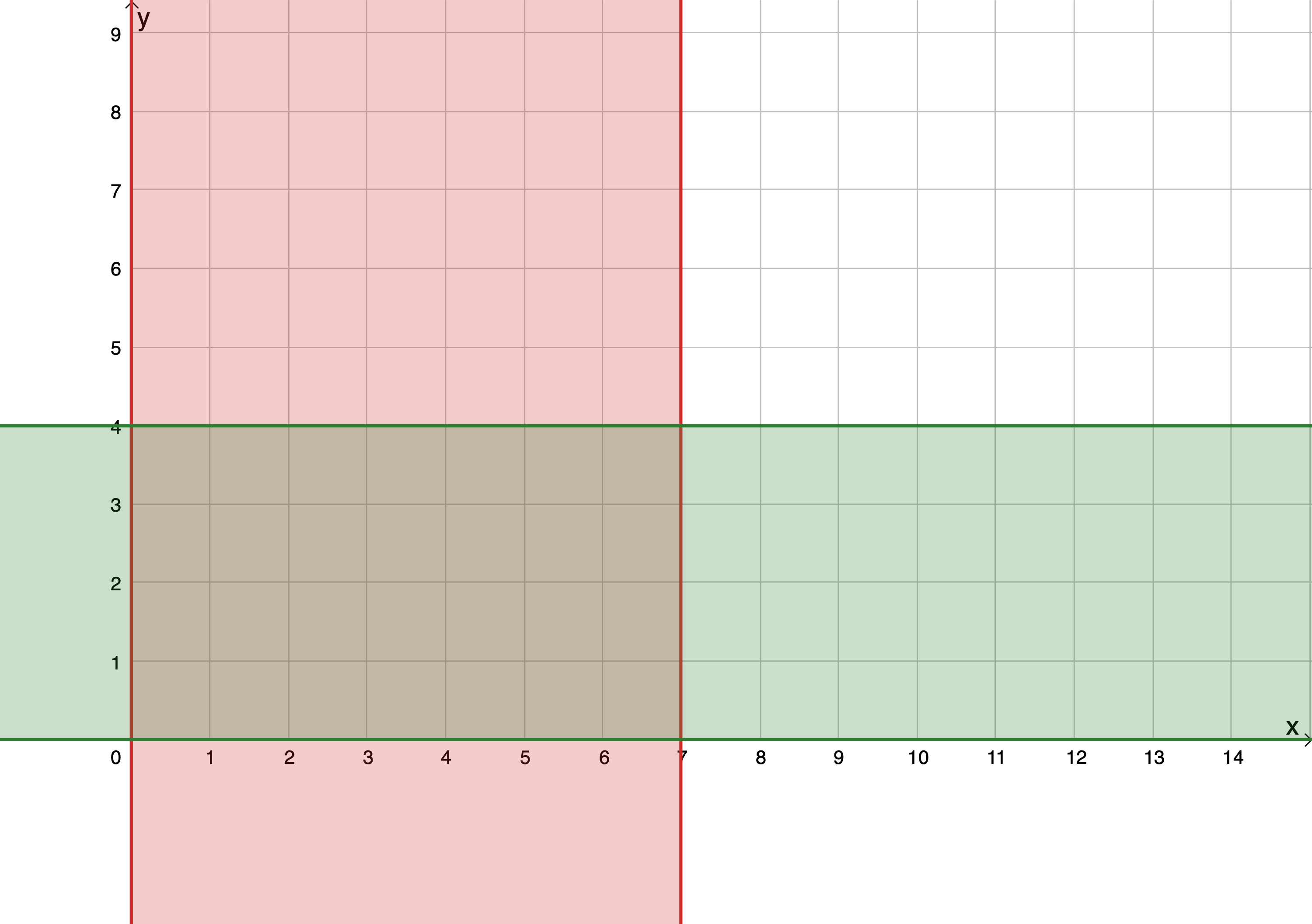
But we have another constraint: [latex]\scriptsize 3x+2y\le 18[/latex].
[latex]\scriptsize \begin{align*}3x+2y & \le 18\\\therefore 2y & \le -3x+18\\\therefore y & \le -\displaystyle \frac{3}{2}x+9\end{align*}[/latex]
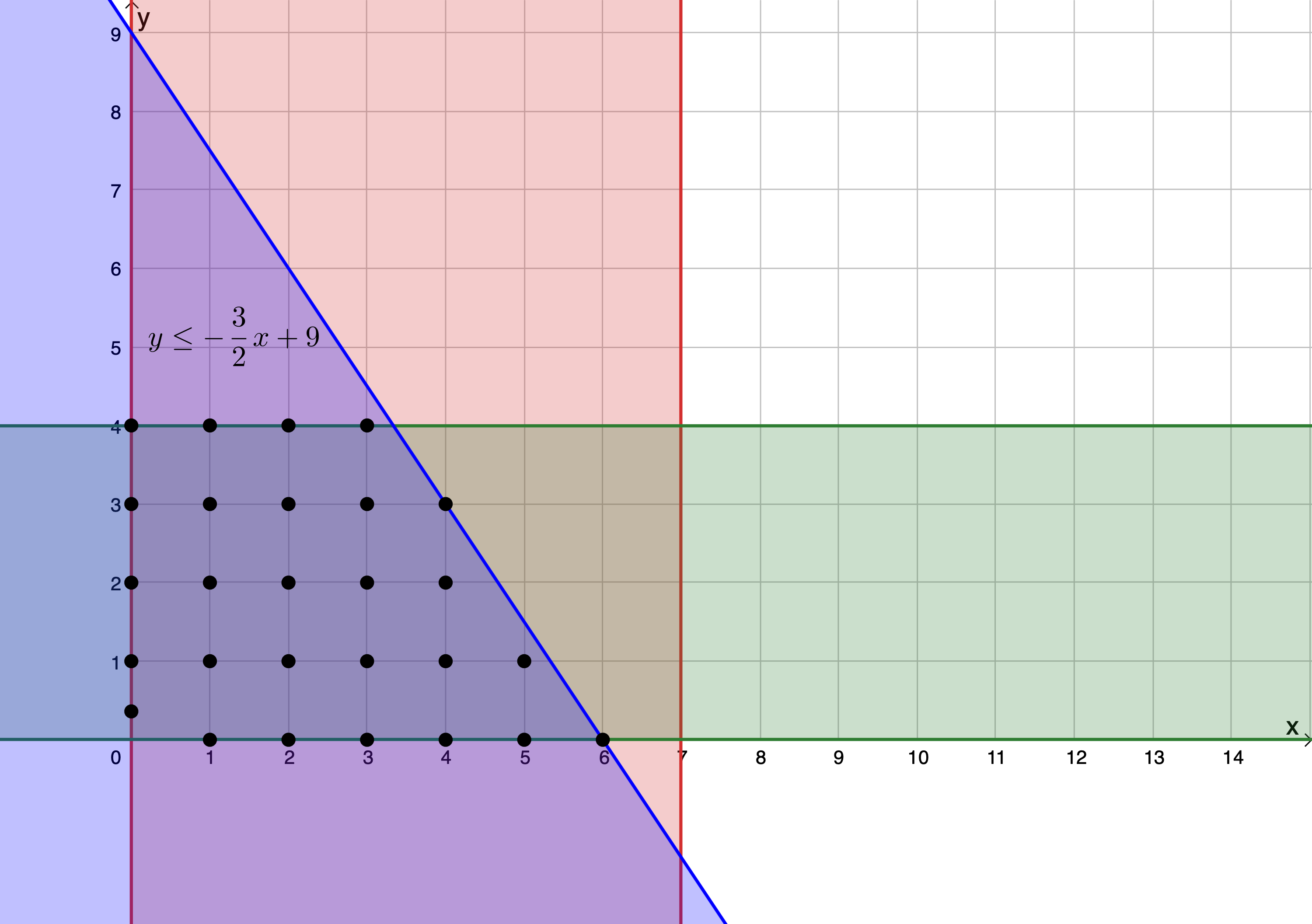
First, we sketch the line [latex]\scriptsize y=-\displaystyle \frac{3}{2}x+9[/latex] and then we shade the region below this line because our constraint is [latex]\scriptsize y\le -\displaystyle \frac{3}{2}x+9[/latex] (see Figure 4). If the constraint was [latex]\scriptsize y\ge -\displaystyle \frac{3}{2}x+9[/latex], we would shade the region above the line.
The region where all three separate regions overlap is called the feasible region. It is in this region that the solution to our problem lies.
We could explicitly show that we are only interested in the natural numbers by plotting these points within the feasible region (see Figure 5).
Step 5: Graph the objective function
Our objective function is [latex]\scriptsize 2\ 400x+1\ 200y=C[/latex].
[latex]\scriptsize \begin{align*}2\ 400x+1\ 200y&=C\\ \therefore 1\ 200y & =-2\ 400x+C\\ \therefore y & =\displaystyle \frac{{-2\ 400}}{{1\ 200}}x+\displaystyle \frac{C}{{1\ 200}}\\ \therefore y&=-2x+\displaystyle \frac{C}{{1\ 200}}\end{align*}[/latex]
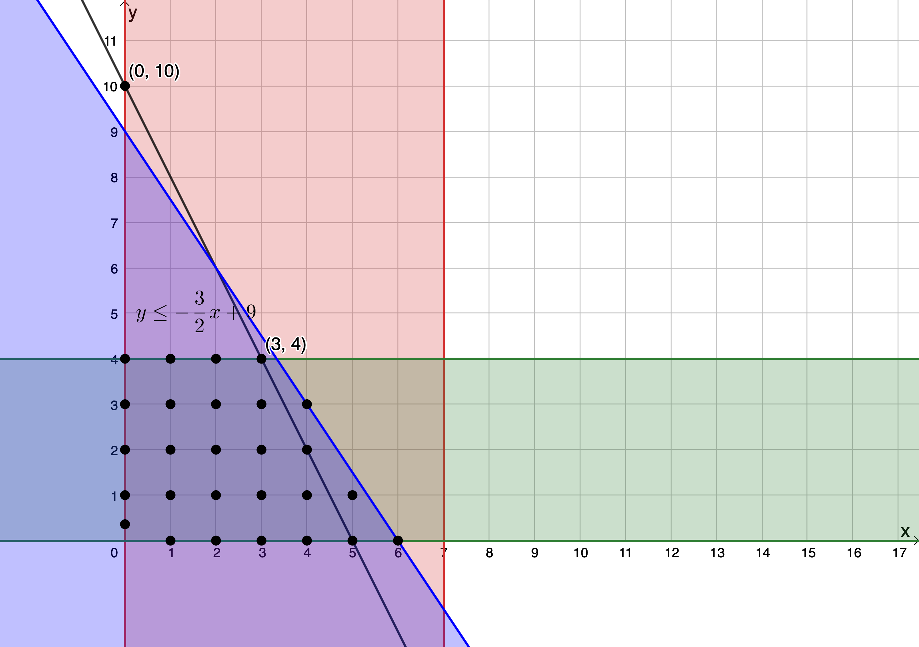
Now we cannot really graph this linear function because we don’t yet know what the value of [latex]\scriptsize C[/latex] is. But remember, [latex]\scriptsize C[/latex] is what we are trying to minimise, for a maximum number of bicycles produced. In other words, we are trying to find the lowest value of [latex]\scriptsize C[/latex] that will make our objective function pass through one of the possible solution points with the largest coordinates within the feasible region.
So, we start with any line with a gradient of [latex]\scriptsize -2[/latex] and move this line up and down to find the smallest y-intercept value that still lets the objective function pass through one of the points in the feasible region with the largest possible [latex]\scriptsize x[/latex] and [latex]\scriptsize y[/latex] coordinates. The objective function must pass through [latex]\scriptsize (3,4)[/latex] for the y-intercept to be a minimum ([latex]\scriptsize 10[/latex]), and [latex]\scriptsize x[/latex] and [latex]\scriptsize y[/latex] to be maximum. The solution is shown below in Figure 6.
Step 6: Answer the questions
We are now in a position to answer the questions.
- Qhubeka must make three Buffalo bicycles and four Cheetah bicycles per day to minimise costs.
- The minimum solution to the objective function results in a y-intercept of [latex]\scriptsize (0,10)[/latex]. The objective function is [latex]\scriptsize y=-2x+\displaystyle \frac{C}{{1\ 200}}\text{ }[/latex]. Therefore:
[latex]\scriptsize \begin{align*}\displaystyle \frac{C}{{1\ 200}} & =10\\\therefore C & =12\ 000\end{align*}[/latex]The minimum cost is [latex]\scriptsize \text{R}12\ 000[/latex].
Note
If you have an internet connection, visit a simulation of this linear programming solution.
There is a slider to change the value of [latex]\scriptsize C[/latex] in order to find the minimum or maximum solution to the objective function.
Let’s look at another example.
Example 1.2
A TVET college class wants to raise funds to help buy new workshop tools. To raise money, they decide to host a cake sale and sell two different types of cakes – chocolate cake and carrot cake.
The class estimates that they can sell at most [latex]\scriptsize 60[/latex] chocolate cakes and [latex]\scriptsize 50[/latex] carrot cakes.
Each chocolate cake takes [latex]\scriptsize 50\ \min[/latex] to bake and each carrot cake takes [latex]\scriptsize 80\ \min[/latex] to bake. In total, the class calculates that they have [latex]\scriptsize 4\ 400\min[/latex] to bake all the cakes.
Each chocolate cake costs [latex]\scriptsize \text{R}30[/latex] to make and each carrot cake costs [latex]\scriptsize \text{R}40[/latex] to make and they have a total of [latex]\scriptsize \text{R2}\ 400[/latex] to spend on ingredients.
They can sell each chocolate cake for [latex]\scriptsize \text{R3}0[/latex] profit and each carrot cake for [latex]\scriptsize \text{R6}0[/latex] profit.
- Assuming they can sell all the cakes they bake, how many of each type of cake should they bake to maximise their profit?
- What will this maximum profit be?
Solution
Step 1: Assign variables
Let the number of chocolate cakes be [latex]\scriptsize x[/latex].
Let the number of carrot cakes be [latex]\scriptsize y[/latex].
We cannot have fractions of cakes or negative numbers of cakes. Therefore [latex]\scriptsize \{x|x\in \mathbb{N}\}\text{ }[/latex] and [latex]\scriptsize \{y|y\in \mathbb{N}\}\text{ }[/latex].
Step 2: Express the constraints
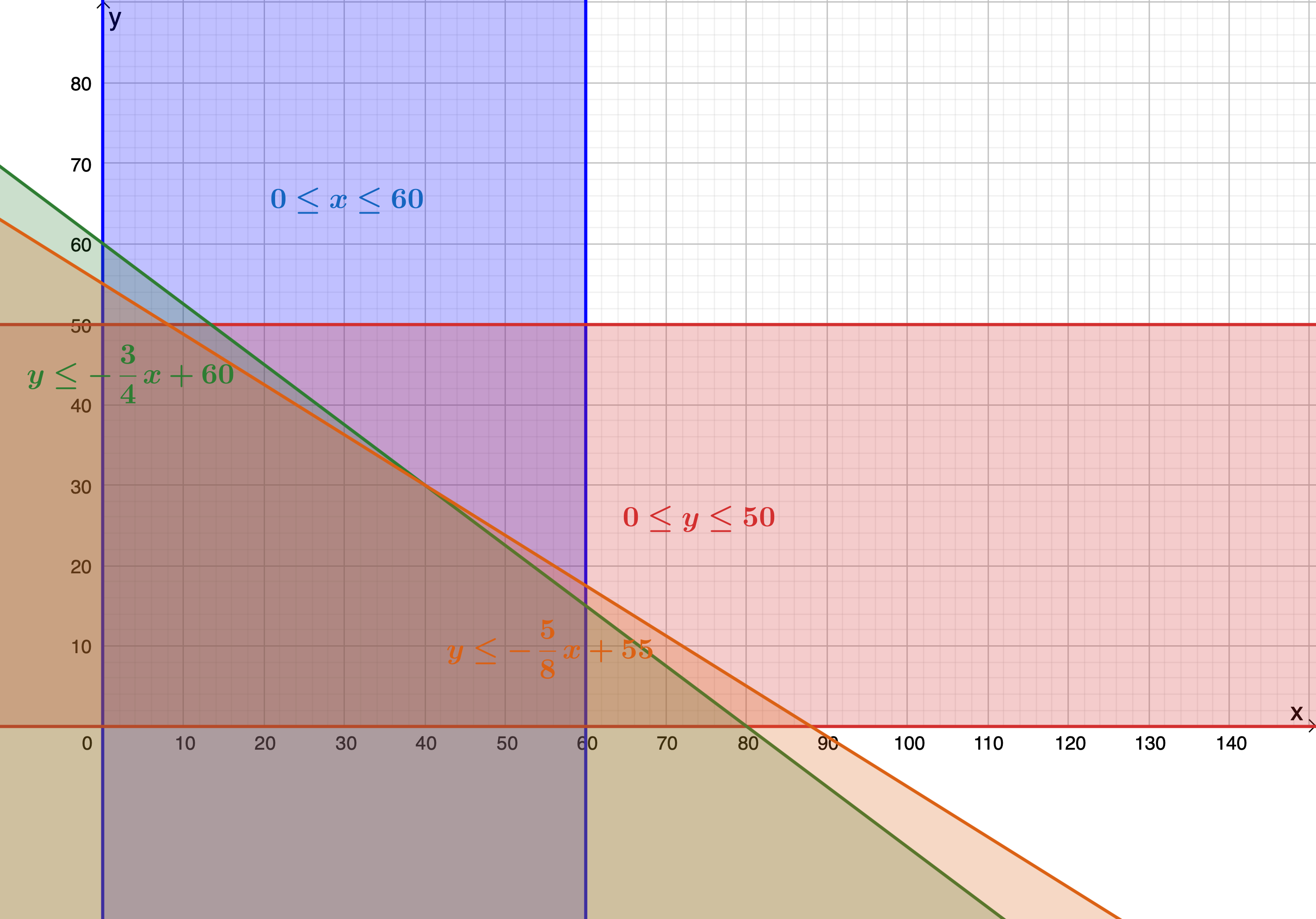
- [latex]\scriptsize x\le 60[/latex] (at most [latex]\scriptsize 60[/latex] chocolate cakes can be sold)
- [latex]\scriptsize y\le 50[/latex] (at most [latex]\scriptsize 50[/latex] carrot cakes can be sold)
- [latex]\scriptsize 50x+80y\le 4\ 400[/latex] (each chocolate cake takes [latex]\scriptsize 50\ \min[/latex] and each carrot cake takes [latex]\scriptsize 80\ \min[/latex] to bake and they have a total of [latex]\scriptsize 4\ 400\ \min[/latex] to bake).
- [latex]\scriptsize 30x+40y=2\ 400[/latex] (each chocolate cake costs [latex]\scriptsize \text{R}30[/latex] and each carrot cake costs [latex]\scriptsize \text{R}40[/latex] and they have a total of [latex]\scriptsize \text{R}2\ 400[/latex] to spend)
Step 3: Determine the objective function
[latex]\scriptsize 30x+60y=P[/latex], where [latex]\scriptsize P[/latex] is profit.
Step 4: Graph the constraints
[latex]\scriptsize \begin{align*}50x+80y\le 4\ 400\\\therefore 80y\le -50x+4\ 400\\\therefore y\le -\displaystyle \frac{{50}}{{80}}x+\displaystyle \frac{{4\ 400}}{{80}}\\\therefore y\le -\displaystyle \frac{5}{8}x+55\end{align*}[/latex]
[latex]\scriptsize \begin{align*}30x+40y & \le 2\ 400\\\therefore 40y & \le -30x+2\ 400\\\therefore y & \le -\displaystyle \frac{{30}}{{40}}x+\displaystyle \frac{{2\ 400}}{{40}}\\\therefore y & \le -\displaystyle \frac{3}{4}x+60\end{align*}[/latex]
The graphed constraints are shown in Figure 7.
Step 5: Graph the objective function
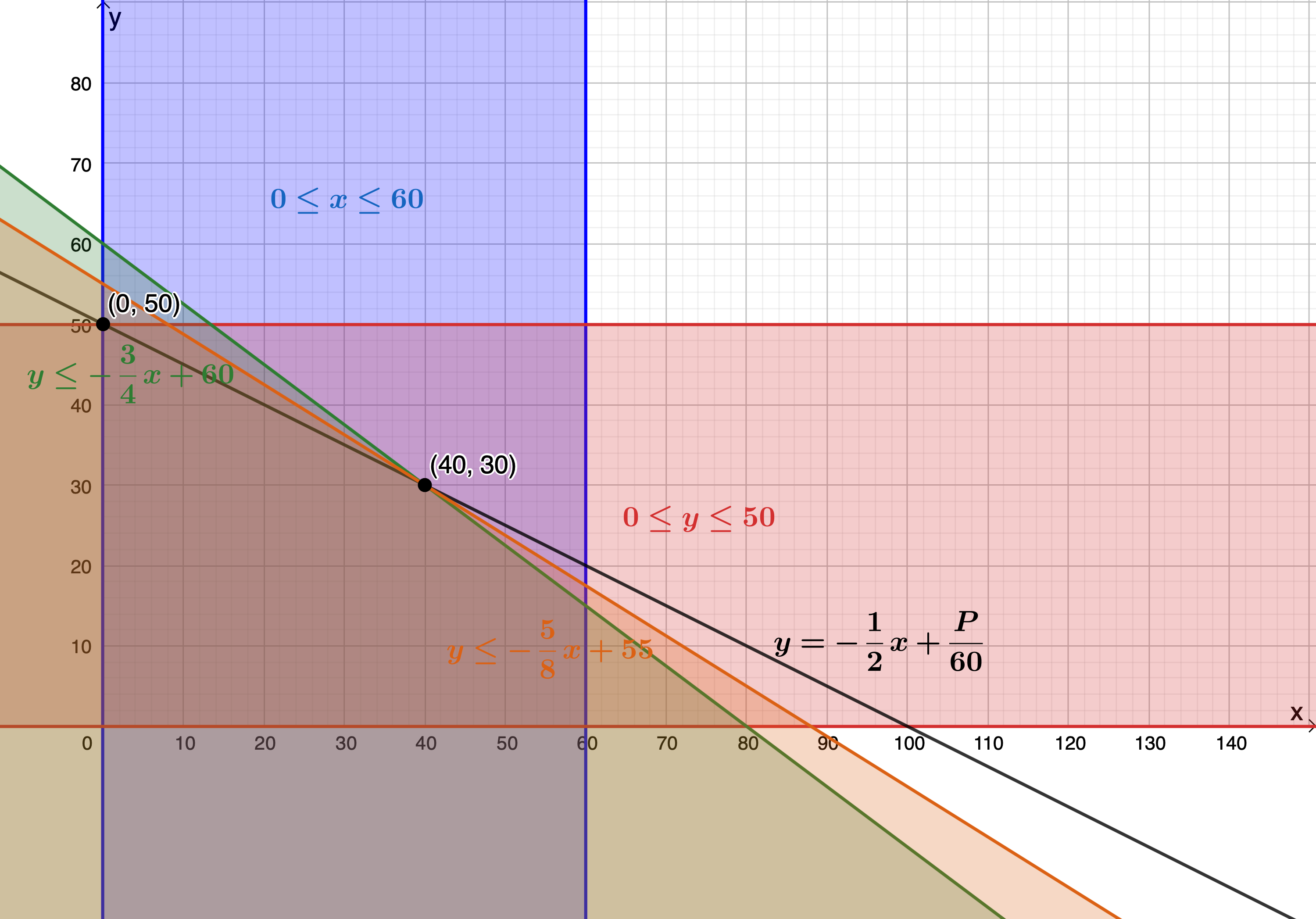
[latex]\scriptsize \begin{align*}30x+60y & =P\\\therefore 60y & =-30x+p\\\therefore y & =-\displaystyle \frac{{30}}{{60}}x+\displaystyle \frac{P}{{60}}\\\therefore y & =-\displaystyle \frac{1}{2}x+\displaystyle \frac{P}{{60}}\end{align*}[/latex]
An instance of the objective function is graphed in Figure 8.
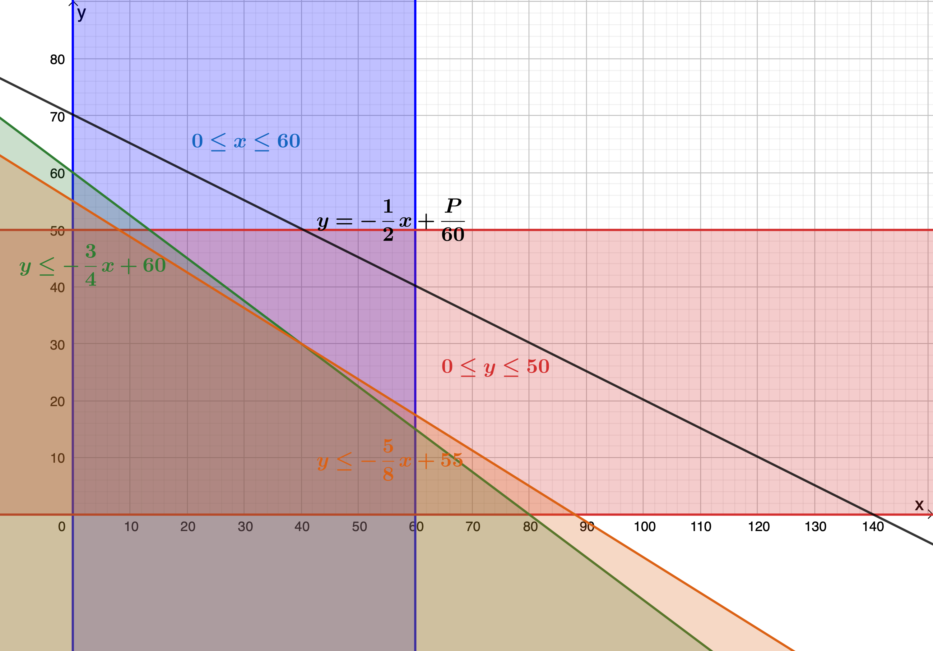
In this case, we want to maximise the objective function, in other words, we want to find the maximum y-intercept that the graph can have while still passing through one of the possible solution points in the feasible region. From the graph of the feasible region, we can see that this point is [latex]\scriptsize (40,30)[/latex]. When the objective function is made to pass through this point its y-intercept is [latex]\scriptsize 50[/latex] (see Figure 9).
Step 6: Answer the questions
- The class should bake [latex]\scriptsize 40[/latex] chocolate cakes and [latex]\scriptsize 30[/latex] carrot cakes to maximise their profit.
- [latex]\scriptsize y=-\displaystyle \frac{1}{2}x+\displaystyle \frac{P}{{60}}[/latex]
[latex]\scriptsize \begin{align*}\displaystyle \frac{P}{{60}} & =50\\\therefore P=3\ 000\end{align*}[/latex]
The maximum profit they can make is [latex]\scriptsize \text{R3}\ 000[/latex].
Exercise 1.1
Question taken from Question 2.3 of NC(V) Mathematics Paper 1 March 2014
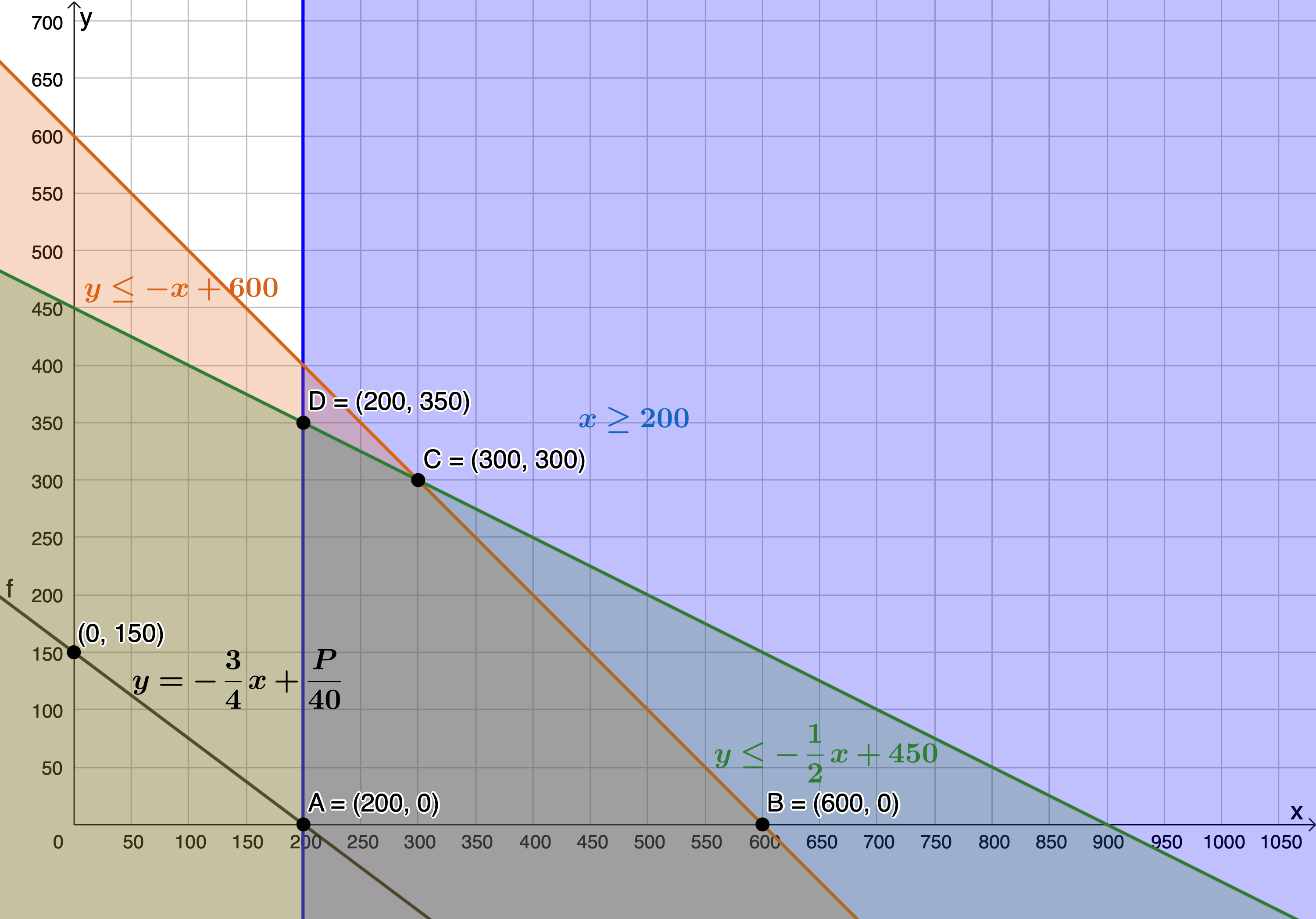
A clothing company manufactures yellow T-shirts ([latex]\scriptsize x[/latex]) and black trousers ([latex]\scriptsize y[/latex]) for a day-care school. The following system of inequalities are obtained:
[latex]\scriptsize x\ge 200[/latex]
[latex]\scriptsize x+y\le 600[/latex]
[latex]\scriptsize x+2y\le 900[/latex]
[latex]\scriptsize 50x+100y\le 45\ 000[/latex]
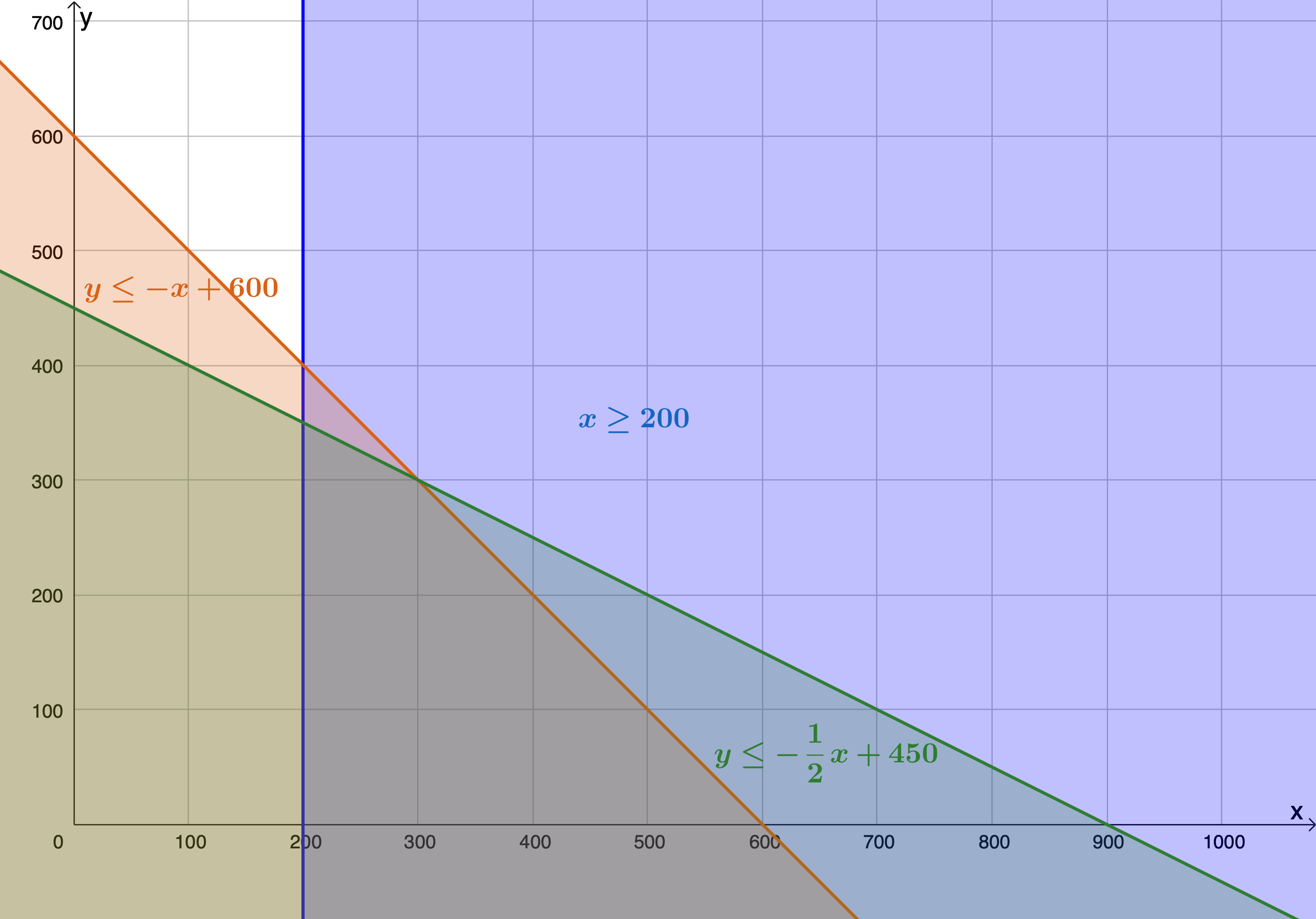
- Sketch the graphs of the given constraints.
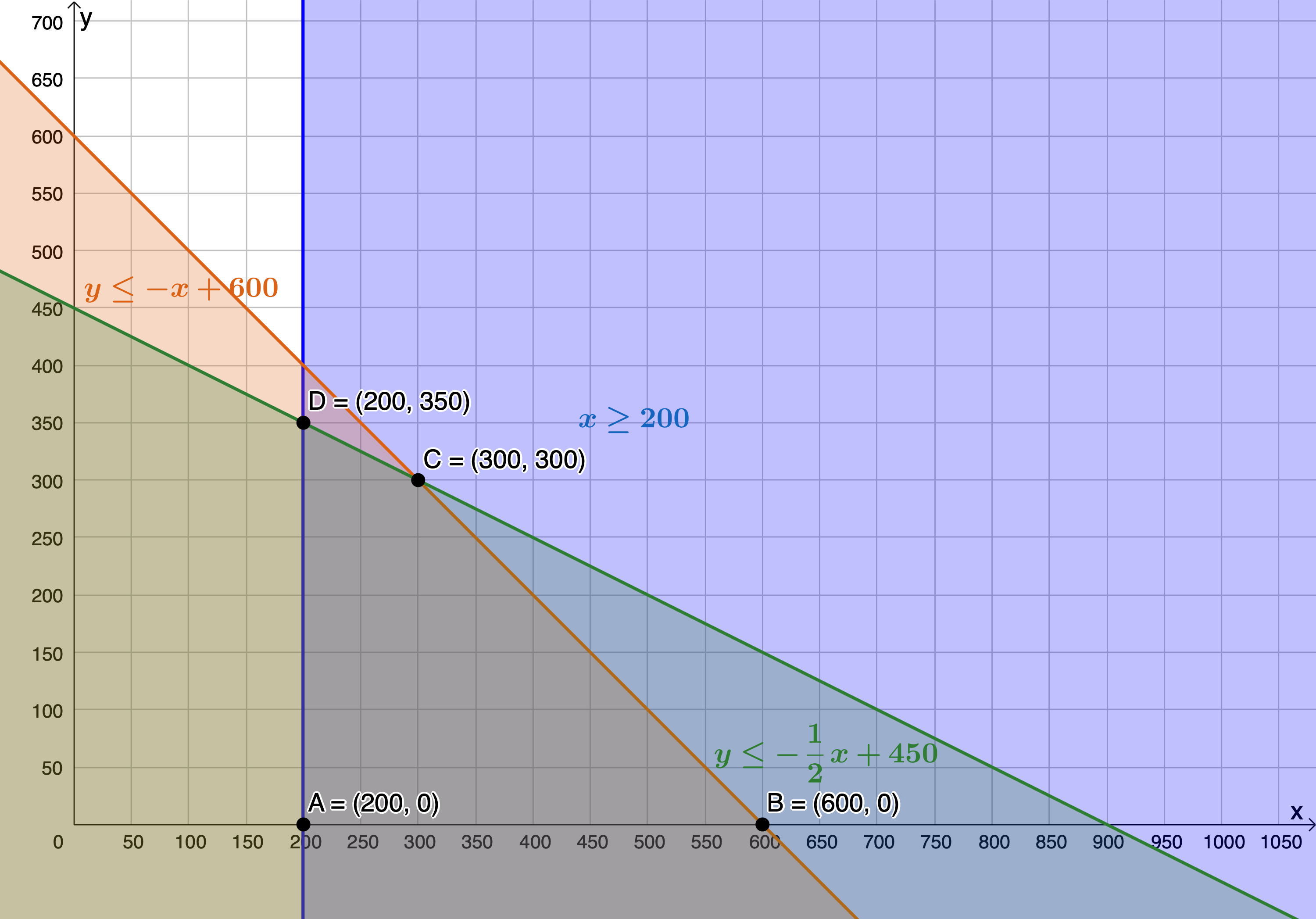
- Indicate the feasible region.
- Determine the number of t-shirts and pairs of trousers that will yield a maximum profit if [latex]\scriptsize P=30x+40y[/latex].
- Determine the number of t-shirts and pairs of trousers that will yield a minimum profit if [latex]\scriptsize P=30x+40y[/latex].
The full solutions are at the end of the unit.
Summary
In this unit you have learnt the following:
- How to express given constraints using variables.
- How to plot these constraints on the Cartesian plane.
- How to determine the feasible region.
- How to determine the objective function.
- How to maximise or minimise the objective function.
Unit 1: Assessment
Suggested time to complete: 15 minutes
Question 1 is based on Question 2.5 from NC(V) Mathematics Paper 1 October 2012
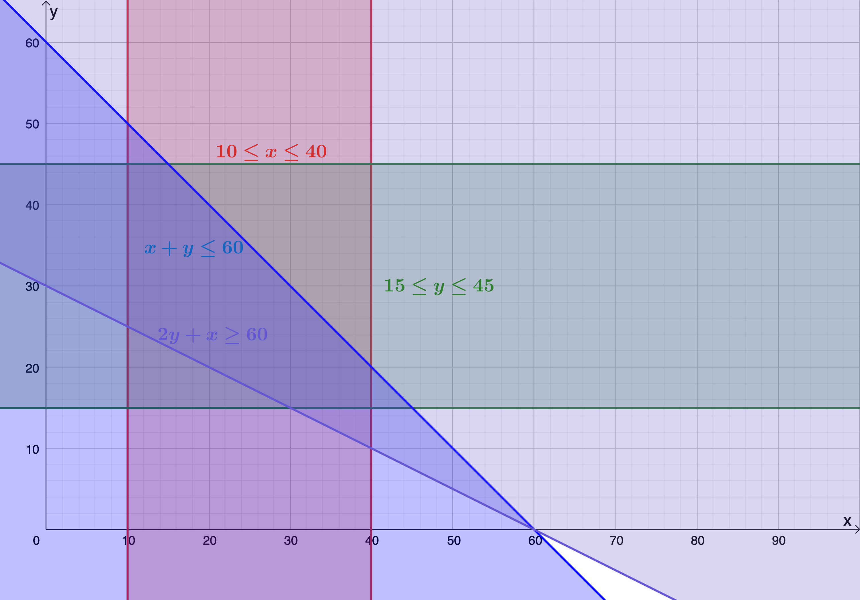
- An entrepreneur sells apples and bananas at the fruit stand. Suppose [latex]\scriptsize x[/latex] apples and [latex]\scriptsize y[/latex] bananas are sold every hour, and that the following constraints are applicable:
[latex]\scriptsize 10\le x\le 40[/latex]
[latex]\scriptsize x+y\le 60[/latex]
[latex]\scriptsize 15\le y\le 45[/latex]
[latex]\scriptsize 2y+x\ge 60[/latex]- Sketch the graph with the given constraints.
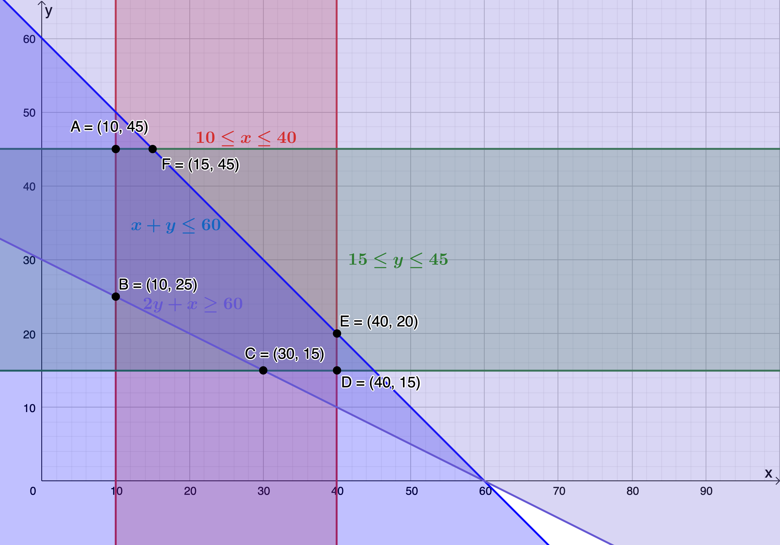
- Determine the feasible region.
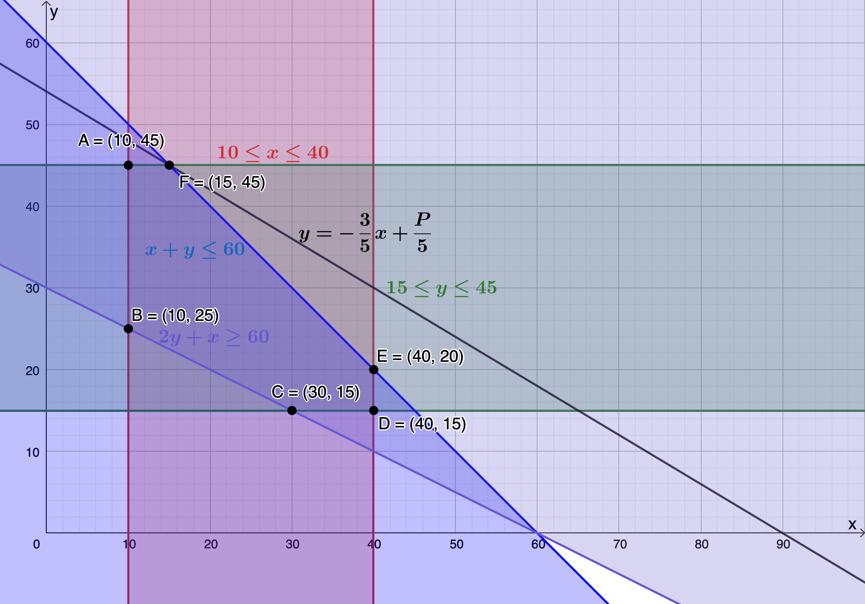
- Determine how many apples and bananas should be sold every hour so that the maximum profit can be made if [latex]\scriptsize P=3x+5y[/latex].
Question 2 is taken from Question 3.3 from NC(V) Mathematics Paper 1 October 2014
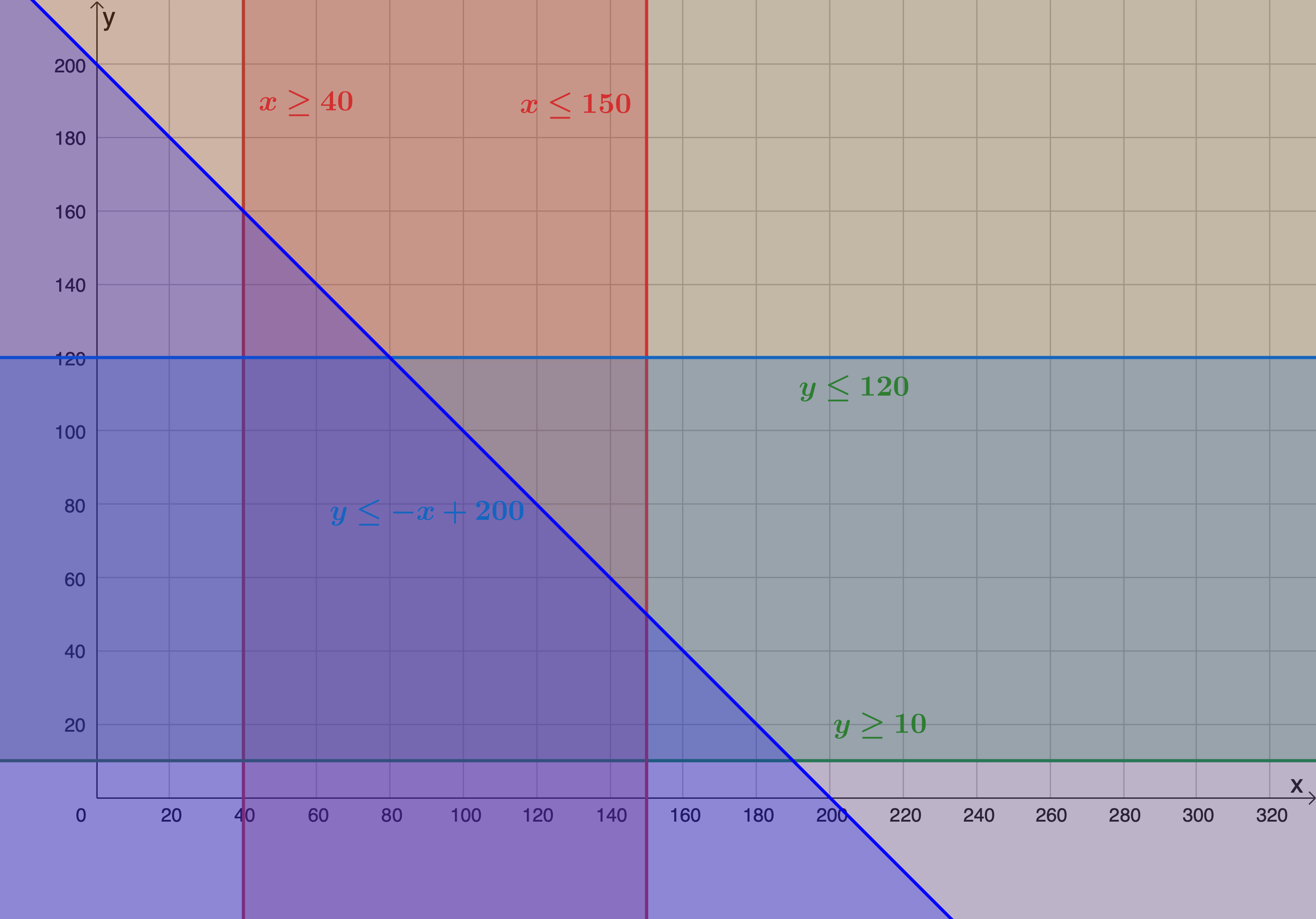
- Lesedi is a small company that makes two types of cards, type A ([latex]\scriptsize x[/latex]) and type B ([latex]\scriptsize y[/latex]). With the available labour and materials, the following are the constraints inequalities:
[latex]\scriptsize x+y\le 200[/latex]
[latex]\scriptsize x\ge 40[/latex]
[latex]\scriptsize y\ge 10[/latex]
[latex]\scriptsize x\le 150[/latex]
[latex]\scriptsize y\le 120[/latex]- Sketch the graph of the given constraints.
- Determine the feasible region.
- Find the values of [latex]\scriptsize x[/latex] and [latex]\scriptsize y[/latex] which will maximise the objective equation [latex]\scriptsize P=5x+10y[/latex].
- Find the values of [latex]\scriptsize x[/latex] and [latex]\scriptsize y[/latex] which will minimise the objective equation [latex]\scriptsize P=5x+10y[/latex] and state the value of [latex]\scriptsize P[/latex] when this function is minimised.
The full solutions are at the end of the unit.
Unit 1: Solutions
Exercise 1.1
- [latex]\scriptsize x\in \mathbb{N}\text{ }[/latex] and [latex]\scriptsize y\in \mathbb{N}\text{ }[/latex]
Constraints are:
[latex]\scriptsize x\ge 200[/latex]
.
[latex]\scriptsize \begin{align*}x+y & \le 600\\\therefore y & \le -x+600\end{align*}[/latex]
.
[latex]\scriptsize \begin{align*}x+2y & \le 900\\\therefore 2y & \le -x+900\\\therefore y & \le -\displaystyle \frac{1}{2}x+450\end{align*}[/latex]
- The feasible region is the region bound by points [latex]\scriptsize \text{A},\text{B},\text{C}[/latex] and [latex]\scriptsize \text{D}[/latex].
- .
[latex]\scriptsize \begin{align*} P&=30x+40y\\ \therefore 40y&=-30x+P\\ \therefore y&=-\displaystyle \frac{3}{4}x+\displaystyle \frac{P}{40} \end{align*}[/latex]
The objective function is maximised when passing through [latex]\scriptsize \text{C}(300,300)[/latex]. Therefore, [latex]\scriptsize 300[/latex] t-shirts and [latex]\scriptsize 300[/latex] pairs of trousers will yield a maximum profit.
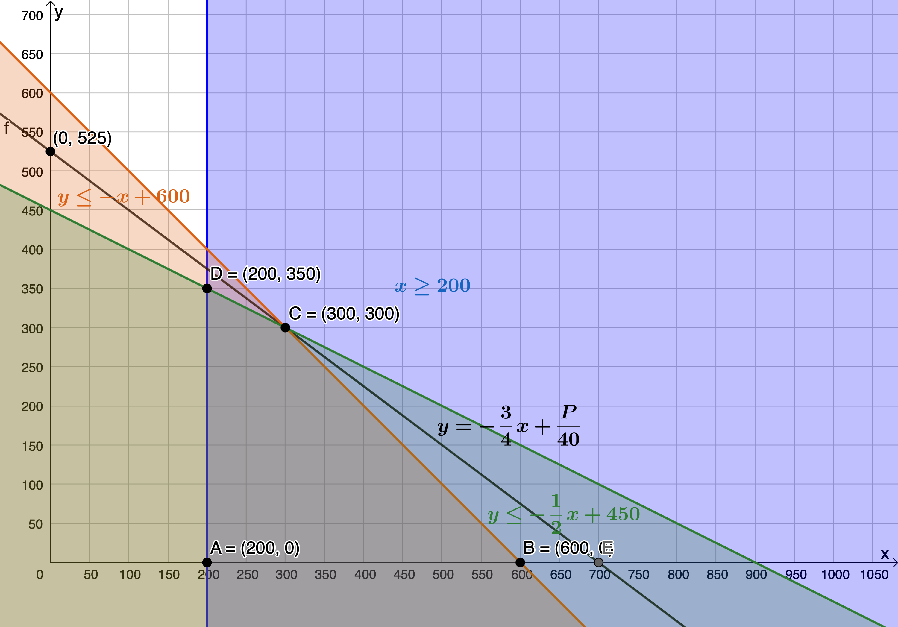
- The objective function is minimised when passing through [latex]\scriptsize \text{A}(200,0)[/latex]. Therefore, [latex]\scriptsize 200[/latex] t-shirts and zero pairs of trousers will yield a minimum profit.
Unit 1: Assessment
- .
- [latex]\scriptsize x\in \mathbb{N}\text{ }[/latex] and [latex]\scriptsize y\in \mathbb{N}\text{ }[/latex]
Constraints are:
[latex]\scriptsize 10\le x\le 40[/latex]
[latex]\scriptsize \begin{align*}x+y & \le 60\\\therefore y & \le -x+60\end{align*}[/latex]
[latex]\scriptsize 15\le y\le 45[/latex]
[latex]\scriptsize \begin{align*}&2y+x\ge 60\\& \therefore y\ge -\displaystyle \frac{1}{2}x+30\quad \text{Remember that because }y\ge \text{ you need to take the region above the line}\end{align*}[/latex]
- The feasible region is the region bound by points [latex]\scriptsize \text{A},\text{B},\text{C},\text{D},\text{E}[/latex] and [latex]\scriptsize \text{F}[/latex].
- .
[latex]\scriptsize \begin{align*} P&=3x+5y\\ \therefore 5y&=-3x+P\\ \therefore y&=-\displaystyle \frac{3}{5}x+\displaystyle \frac{P}{5} \end{align*}[/latex]
The objective function is maximised when passing through [latex]\scriptsize \text{F}(15,45)[/latex]. Therefore, selling [latex]\scriptsize 15[/latex] apples and [latex]\scriptsize 45[/latex] bananas will yield a maximum profit.
- [latex]\scriptsize x\in \mathbb{N}\text{ }[/latex] and [latex]\scriptsize y\in \mathbb{N}\text{ }[/latex]
- .
- [latex]\scriptsize x\in \mathbb{N}\text{ }[/latex] and [latex]\scriptsize y\in \mathbb{N}\text{ }[/latex]
Constraints are:
[latex]\scriptsize \begin{align*}x+y & \le 200\\\therefore y & \le -x+200\end{align*}[/latex]
[latex]\scriptsize x\ge 40[/latex]
[latex]\scriptsize y\ge 10[/latex]
[latex]\scriptsize x\le 150[/latex]
[latex]\scriptsize y\le 120[/latex]
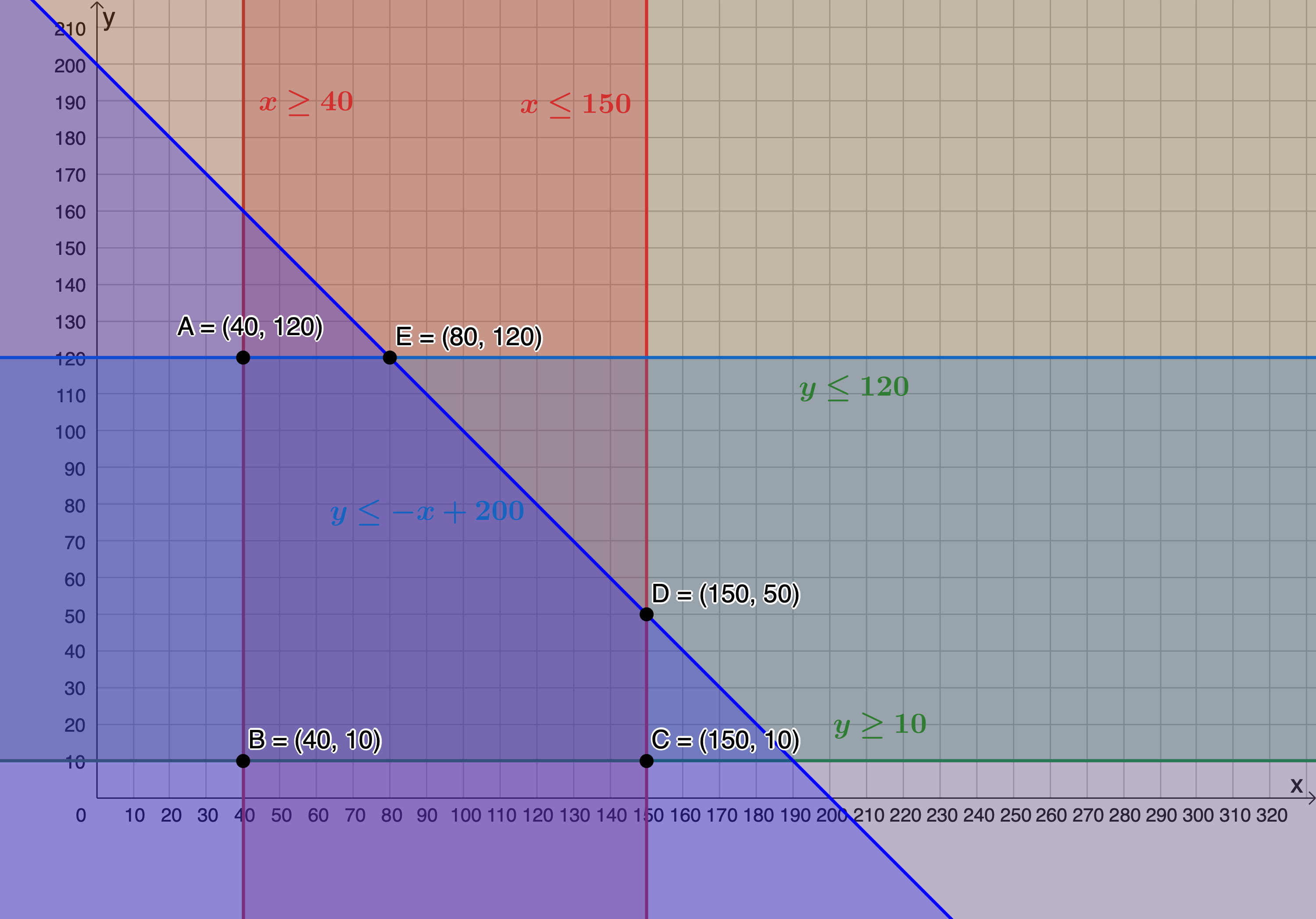
- The feasible region is the region bound by points [latex]\scriptsize \displaystyle \text{A},\text{B},\text{C},\text{D}[/latex] and [latex]\scriptsize \text{E}[/latex].
- .
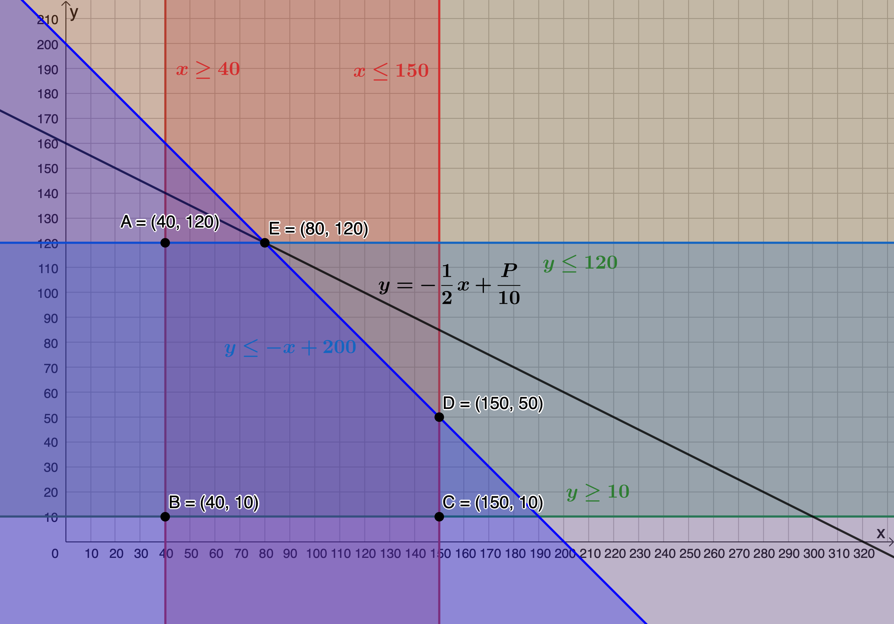
[latex]\scriptsize \begin{align*} P&=5x+10y\\ \therefore 10y&=-5x+P\\ \therefore y&=-\displaystyle \frac{1}{2}x+\displaystyle \frac{P}{10} \end{align*}[/latex]
The objective function is maximised when passing through [latex]\scriptsize \text{E}(80,120)[/latex]. Therefore, [latex]\scriptsize x=80[/latex] and [latex]\scriptsize y=120[/latex].
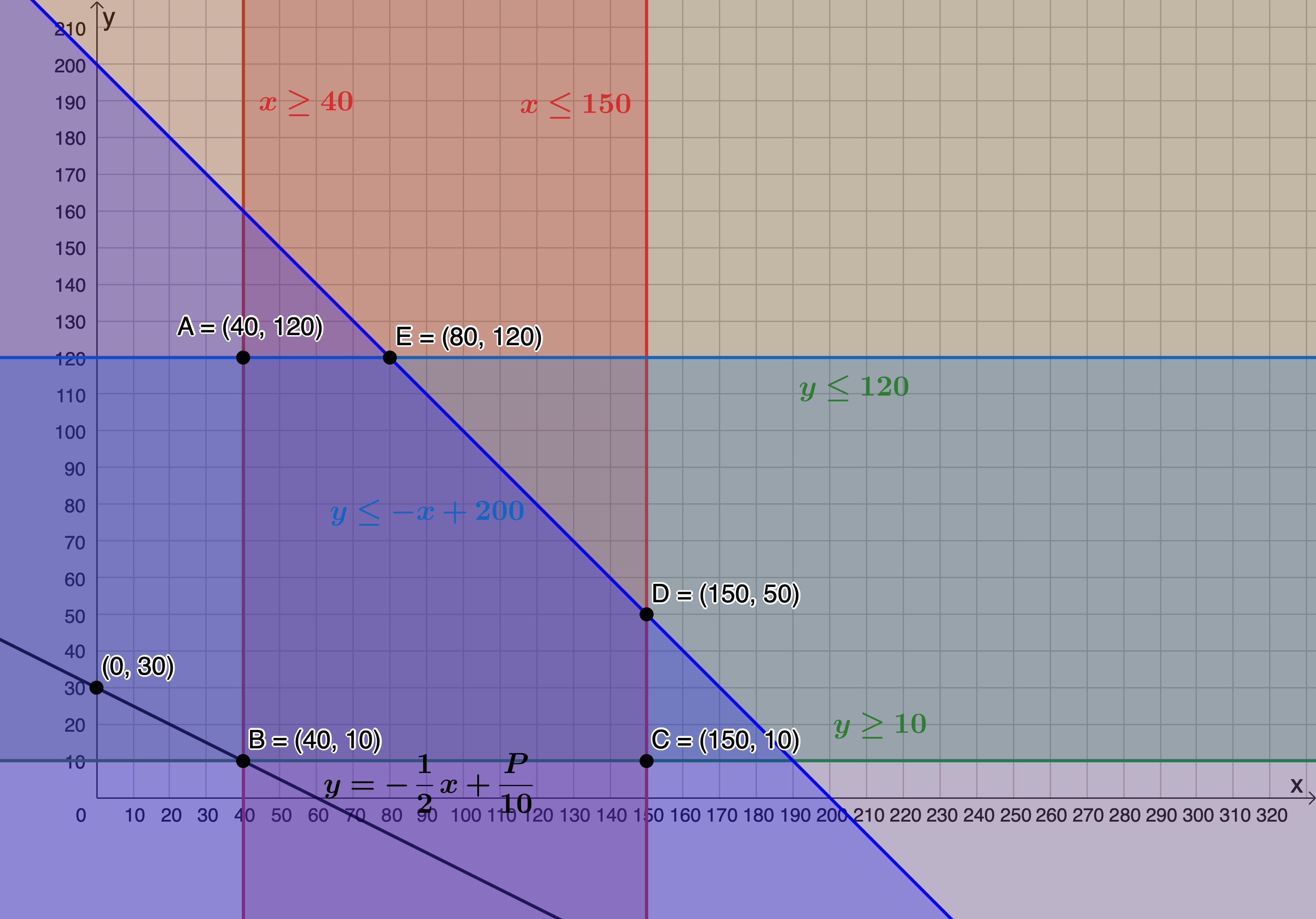
- The objective function is minimised when passing through [latex]\scriptsize \text{B}(40,10)[/latex]. Therefore, [latex]\scriptsize x=40[/latex] and [latex]\scriptsize y=10[/latex]. When minimised, the objective function has a y-intercept of [latex]\scriptsize (0,30)[/latex].
[latex]\scriptsize \begin{align*}\displaystyle \frac{P}{{10}} & =30\\\therefore P & =300\end{align*}[/latex]
Therefore [latex]\scriptsize P=300[/latex] is the value of [latex]\scriptsize P[/latex] when the function is minimised.
- [latex]\scriptsize x\in \mathbb{N}\text{ }[/latex] and [latex]\scriptsize y\in \mathbb{N}\text{ }[/latex]
Media Attributions
- figure1 © Qhubeka is licensed under a All Rights Reserved license
- figure2 © Geogebra is licensed under a CC BY-SA (Attribution ShareAlike) license
- figure3 © Geogebra is licensed under a CC BY-SA (Attribution ShareAlike) license
- figure4 © Geogebra is licensed under a CC BY-SA (Attribution ShareAlike) license
- figure5 © Geogebra is licensed under a CC BY-SA (Attribution ShareAlike) license
- figure6 © Geogebra is licensed under a CC BY-SA (Attribution ShareAlike) license
- figure7 © Geogebra is licensed under a CC BY-SA (Attribution ShareAlike) license
- figure8 © Geogebra is licensed under a CC BY-SA (Attribution ShareAlike) license
- figure9 © Geogebra is licensed under a CC BY-SA (Attribution ShareAlike) license
- exercise1.1A1 © Geogebra is licensed under a CC BY-SA (Attribution ShareAlike) license
- exercise1.1A2 © Geogebra is licensed under a CC BY-SA (Attribution ShareAlike) license
- exercise1.1A3 © Geogebra is licensed under a CC BY-SA (Attribution ShareAlike) license
- exercise1.1A4 © Geogebra is licensed under a CC BY-SA (Attribution ShareAlike) license
- assessmentA1a © Geogebra is licensed under a CC BY-SA (Attribution ShareAlike) license
- assessmentA1b © Geogebra is licensed under a CC BY-SA (Attribution ShareAlike) license
- assessmentA1c © Geogebra is licensed under a CC BY-SA (Attribution ShareAlike) license
- assessmentA2a © Geogebra is licensed under a CC BY-SA (Attribution ShareAlike) license
- assessmentA2b © Geogebra is licensed under a CC BY (Attribution) license
- assessmentA2c © Geogebra is licensed under a CC BY-SA (Attribution ShareAlike) license
- assessmentA2d © Geogebra is licensed under a CC BY-SA (Attribution ShareAlike) license
