Data handling: Calculate, represent and interpret measures of central tendency and dispersion in univariate numerical grouped data
Unit 2: Construct the ogive
Natashia Bearam-Edmunds
Unit outcomes
By the end of this unit you will be able to:
- Work out class intervals.
- Plot the ogive.
- Interpret the ogive.
What you should know
Before you start this unit, make sure you can:
- Construct a frequency distribution. Work through unit 1 of this subject outcome if you need to revise frequency distributions.
Introduction
In unit 1 of this subject outcome we learnt that when consecutive frequencies are added together we get cumulative frequencies. A cumulative frequency can be plotted as its own graph, called the ogive (pronounced ‘o-jive’) or the cumulative frequency graph. We use the data and intervals from a grouped frequency distribution to plot the ogive. As you will see it is easier to get information by looking at an ogive rather than working through the data in a frequency table.
The ogive is used to approximate the number of observations less than or equal to a specific value and is useful when you want to see what has happened up to a particular point. The following activity will take you through the process of constructing an ogive.
Activity 2.1: Use a frequency distribution to draw an ogive
Time required: 20 minutes
What you need:
- a pen and paper
What to do:
Below is the cumulative frequency table of the ages of people attending a public reading by an author at a library.
| Class intervals | Class midpoint | Frequency | Cumulative frequency |
| [latex]\scriptsize 9 \lt x\le 12[/latex] | [latex]\scriptsize \displaystyle 10.5[/latex] | [latex]\scriptsize \displaystyle 5[/latex] | |
| [latex]\scriptsize 12 \lt x\le 15[/latex] | [latex]\scriptsize \displaystyle 8[/latex] | [latex]\scriptsize \displaystyle 13[/latex] | |
| [latex]\scriptsize 15 \lt x\le 18[/latex] | [latex]\scriptsize \displaystyle 13[/latex] | ||
| [latex]\scriptsize 18 \lt x\le 21[/latex] | [latex]\scriptsize \displaystyle 15[/latex] | [latex]\scriptsize \displaystyle 41[/latex] | |
| [latex]\scriptsize 21 \lt x\le 24[/latex] | [latex]\scriptsize \displaystyle 22.5[/latex] | [latex]\scriptsize \displaystyle 24[/latex] | |
| [latex]\scriptsize 24 \lt x\le 27[/latex] | [latex]\scriptsize \displaystyle 17[/latex] | [latex]\scriptsize \displaystyle 82[/latex] | |
| [latex]\scriptsize 27 \lt x\le 30[/latex] | [latex]\scriptsize \displaystyle 18[/latex] |
- Rewrite and complete the table.
- If you were to plot a graph of the data, what values would go on the horizontal axis and on the vertical axis?
- How can you make sure the graph starts from the x-axis?
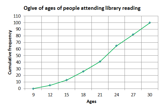
- On a set of labelled axes plot the cumulative frequency against the class midpoints and name your graph.
- What percentage of attendees was less than [latex]\scriptsize \displaystyle 21[/latex] years old?
What did you find?
- Find the class midpoint by adding the lower and upper class limits and dividing by [latex]\scriptsize 2[/latex]. Your completed table should have the following values. You will not use the class midpoint to construct the ogive but it will be useful when we calculate central tendency and dispersion in later units.
Class intervals Class midpoint Frequency Cumulative frequency [latex]\scriptsize 9 \lt x\le 12[/latex] [latex]\scriptsize \displaystyle 10.5[/latex] [latex]\scriptsize \displaystyle 5[/latex] [latex]\scriptsize \displaystyle 5[/latex] [latex]\scriptsize 12 \lt x\le 15[/latex] [latex]\scriptsize \displaystyle 13.5[/latex] [latex]\scriptsize \displaystyle 8[/latex] [latex]\scriptsize \displaystyle 13[/latex] [latex]\scriptsize 15 \lt x\le 18[/latex] [latex]\scriptsize \displaystyle 16.5[/latex] [latex]\scriptsize \displaystyle 13[/latex] [latex]\scriptsize \displaystyle \mathbf{26}[/latex] [latex]\scriptsize 18 \lt x\le 21[/latex] [latex]\scriptsize \displaystyle 19.5[/latex] [latex]\scriptsize \displaystyle 15[/latex] [latex]\scriptsize \displaystyle 41[/latex] [latex]\scriptsize 21 \lt x\le 24[/latex] [latex]\scriptsize \displaystyle 22.5[/latex] [latex]\scriptsize \displaystyle 24[/latex] [latex]\scriptsize \displaystyle \mathbf{65}[/latex] [latex]\scriptsize 24 \lt x\le 27[/latex] [latex]\scriptsize \displaystyle 25.5[/latex] [latex]\scriptsize \displaystyle 17[/latex] [latex]\scriptsize \displaystyle 82[/latex] [latex]\scriptsize 27 \lt x\le 30[/latex] [latex]\scriptsize \displaystyle 28.5[/latex] [latex]\scriptsize \displaystyle 18[/latex] [latex]\scriptsize \displaystyle 100[/latex] To determine the cumulative frequency, we add up the frequencies going down the table. The first cumulative frequency is the same as the frequency, because we are adding it to zero. The final cumulative frequency is always equal to the sum of all the frequencies.
- Class intervals in numbers of years is plotted on the x-axis and cumulative frequency plotted on the vertical axis (y-axis).
- For the graph to start on the x-axis, the first lower class boundary must be plotted with a cumulative frequency of zero. There are no data values between zero and [latex]\scriptsize \displaystyle 9[/latex] so the graph must reflect no data values in that range.
- Plot a dot at each class interval endpoint against the cumulative frequency. Join the dots using line segments.
- Read off from the graph as shown below. Find [latex]\scriptsize 21[/latex] on the x-axis and draw a vertical line upward until you touch the ogive, then draw a horizontal line from that point to meet the y-axis. The corresponding value on the y-axis tells you how many people were less than [latex]\scriptsize 21[/latex].
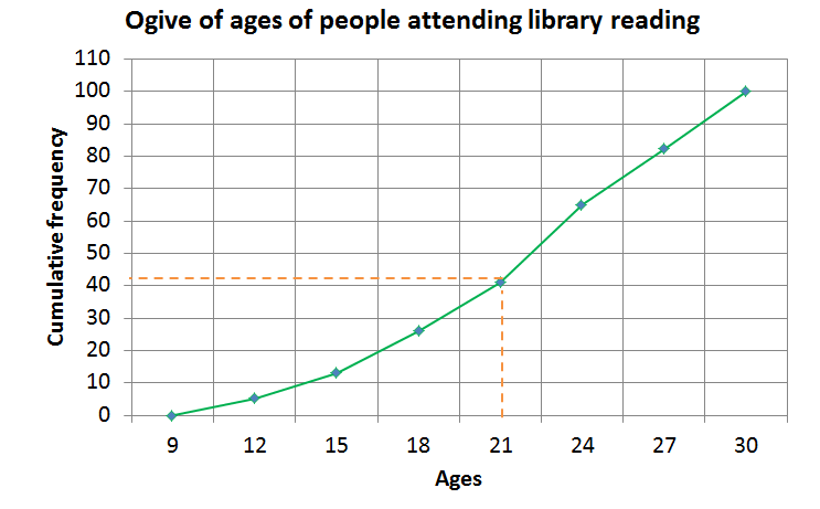
We see that [latex]\scriptsize \displaystyle \displaystyle \frac{{41}}{{100}}=41\%[/latex] of attendees were less than [latex]\scriptsize \displaystyle 21[/latex] years old.
How to construct a cumulative frequency graph/ogive
In Activity 2.1 we saw that these are the steps to construct an ogive:
- The class intervals are labelled on the horizontal axis (x-axis) and the cumulative frequencies along the vertical axis (y-axis).
- Every ogive will start at the lower boundary of the first-class interval on the horizontal axis with a frequency of zero.
- Plot a dot at each class interval endpoint against the cumulative frequency. In this way, the end of the final interval will always be the total number of data elements that we will have added up across all intervals.
- Join the dots using straight lines.
Note: this is not a continuous curve.
Example 2.1
- The table shows the marks out of [latex]\scriptsize 60[/latex] for a physics test.
Complete the table.Intervals Frequency Cumulative frequency [latex]\scriptsize 10 \lt n\le 20[/latex] [latex]\scriptsize 5[/latex] [latex]\scriptsize 20 \lt n\le 30[/latex] [latex]\scriptsize 7[/latex] [latex]\scriptsize 30 \lt n\le 40[/latex] [latex]\scriptsize 12[/latex] [latex]\scriptsize 40 \lt n\le 50[/latex] [latex]\scriptsize 10[/latex] [latex]\scriptsize 50 \lt n\le 60[/latex] [latex]\scriptsize 6[/latex] - Draw the ogive for the data.
- What percentage of learners got a mark higher than [latex]\scriptsize 40[/latex]?
Solution
- We complete the cumulative frequency column by adding frequencies as we go down the table. The completed table looks like this:
Intervals Frequency Cumulative frequency [latex]\scriptsize 10 \lt n\le 20[/latex] [latex]\scriptsize 5[/latex] [latex]\scriptsize 5[/latex] [latex]\scriptsize 20 \lt n\le 30[/latex] [latex]\scriptsize 7[/latex] [latex]\scriptsize 12[/latex] [latex]\scriptsize 30 \lt n\le 40[/latex] [latex]\scriptsize 12[/latex] [latex]\scriptsize 24[/latex] [latex]\scriptsize 40 \lt n\le 50[/latex] [latex]\scriptsize 10[/latex] [latex]\scriptsize 34[/latex] [latex]\scriptsize 50 \lt n\le 60[/latex] [latex]\scriptsize 6[/latex] [latex]\scriptsize 40[/latex] - Now we use the completed frequency table to draw the ogive by plotting the endpoint of each interval against the cumulative frequency for that interval.
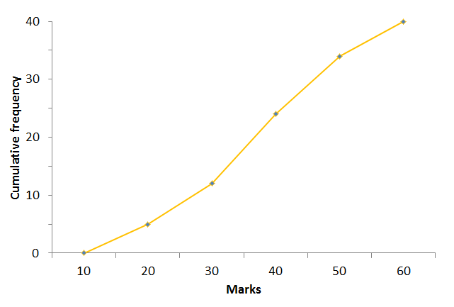
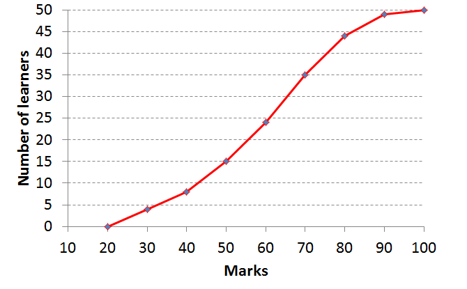
- Find [latex]\scriptsize 40[/latex] on the x-axis and draw a vertical line to meet the ogive, all values to the right of that point are marks that are higher than [latex]\scriptsize 40[/latex]. We can see that [latex]\scriptsize 16[/latex] learners [latex]\scriptsize (40-24)=16[/latex] scored [latex]\scriptsize 40[/latex] or more marks. So [latex]\scriptsize \displaystyle \frac{{16}}{{40}}\times 100=40\%[/latex] of learners got more than [latex]\scriptsize 40[/latex] on the test.
Interpreting the ogive
Ogives are useful for determining the quartiles and five-number summary of data. Remember that the median is simply the value in the middle when we order the data. A quartile is simply a quarter of the way from the beginning or the end of an ordered data set. With an ogive we already know how many data values are above or below a certain point, so it is easy to find the middle or a quarter of the data set. Remember that the answers you find for the quartiles will be approximations as you are dealing with grouped data.
Example 2.2
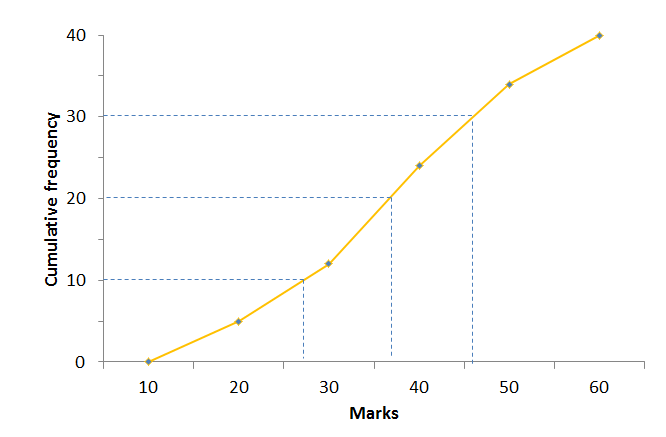
Use the following ogive to compute the five-number summary:
Solution
Remember that the five-number summary consists of the minimum, all the quartiles including the median, which is the second quartile, and the maximum value.
Step 1: Find the minimum and maximum
The minimum value in the data set is [latex]\scriptsize 10[/latex] as this is where the ogive starts on the horizontal axis. The maximum value in the data set is [latex]\scriptsize 60[/latex] as this is where the ogive stops on the horizontal axis.
Step 2: Find the quartiles
The quartiles are the values that are [latex]\scriptsize \displaystyle \frac{1}{4}[/latex] , [latex]\scriptsize \displaystyle \frac{1}{2}[/latex] and [latex]\scriptsize \displaystyle \frac{3}{4}[/latex] of the way into the ordered data set. Here the cumulative frequency goes up to [latex]\scriptsize 40[/latex], so we can find the quartiles by looking at the values corresponding to counts of [latex]\scriptsize 10\text{ }(\displaystyle \frac{1}{4}\times 40)[/latex], [latex]\scriptsize 20\text{ }(\displaystyle \frac{1}{2}\times 40)[/latex] and [latex]\scriptsize 30\text{ }(\displaystyle \frac{3}{4}\times 40)[/latex]. On the ogive, a count of:
- [latex]\scriptsize 10[/latex] corresponds to a value of approximately [latex]\scriptsize 26[/latex] (first quartile)
- [latex]\scriptsize 20[/latex] corresponds to a value of approximately [latex]\scriptsize 36[/latex] (median)
- [latex]\scriptsize 30[/latex] corresponds to a value of approximately [latex]\scriptsize 45[/latex] (third quartile).
Step 3: Write down the five-number summary
[latex]\scriptsize \displaystyle \text{Minimum}=10[/latex]
[latex]\scriptsize {{\text{Q}}_{1}}\approx 26[/latex]
[latex]\scriptsize {{\text{Q}}_{2}}\approx 36[/latex]
[latex]\scriptsize {{\text{Q}}_{3}}\approx 45[/latex]
[latex]\scriptsize \displaystyle \text{Maximum}=60[/latex]
Exercise 2.1
- The following data set lists the ages of [latex]\scriptsize \displaystyle 24[/latex] people.
[latex]\scriptsize \displaystyle \begin{align*}&2;\text{ }5;\text{ }1;\text{ }76;\text{ }34;\text{ }23;\text{ }65;\text{ }22;\text{ }63;\text{ }45;\text{ }53;\text{ }38\\&4;\text{ }28;\text{ }5;\text{ }73;\text{ }79;\text{ }17;\text{ }15;\text{ }5;\text{ }34;\text{ }37;\text{ }45;\text{ }56\end{align*}[/latex]
Use the data to answer the following questions:- Using an interval width of [latex]\scriptsize 8[/latex], construct a cumulative frequency plot.
- Below what value do the bottom [latex]\scriptsize \displaystyle 50\%[/latex] of the ages fall? Give a reason for your answer.
- Below what value do the bottom [latex]\scriptsize \displaystyle 40\%[/latex] fall?
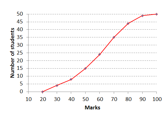
- Use the ogive to answer the questions below. Note that marks are given as a percentage.
- How many learners got between [latex]\scriptsize \displaystyle 50\%[/latex] and [latex]\scriptsize \displaystyle 70\%[/latex]?
- How many learners got at least [latex]\scriptsize \displaystyle 70\%[/latex]?
- Find the median mark for this class, rounded to the nearest integer.
The full solutions are at the end of the unit.
Summary
In this unit you have learnt the following:
- How to construct the ogive from a grouped frequency distribution.
- How to interpret information from an ogive.
Unit 2: Assessment
Suggested time to complete: 25 minutes
- The marks (as a percentage) obtained in an NCV Maths level 3 examination are shown in the table below:
Intervals Frequency Cumulative frequency [latex]\scriptsize \displaystyle ~0 \lt x\le 10[/latex] [latex]\scriptsize \displaystyle 0[/latex] [latex]\scriptsize \displaystyle 0[/latex] [latex]\scriptsize \displaystyle 10 \lt x\le 20[/latex] [latex]\scriptsize \displaystyle 2[/latex] [latex]\scriptsize \displaystyle 20 \lt x\le 30[/latex] [latex]\scriptsize \displaystyle 6[/latex] [latex]\scriptsize \displaystyle 8[/latex] [latex]\scriptsize \displaystyle 30 \lt x\le 40[/latex] [latex]\scriptsize \displaystyle 7[/latex] [latex]\scriptsize \displaystyle 40 \lt x\le 50[/latex] [latex]\scriptsize \displaystyle 14[/latex] [latex]\scriptsize \displaystyle 29[/latex] [latex]\scriptsize \displaystyle 50 \lt x\le 60[/latex] [latex]\scriptsize \displaystyle 20[/latex] [latex]\scriptsize \displaystyle 60 \lt x\le 70[/latex] [latex]\scriptsize \displaystyle 35[/latex] [latex]\scriptsize \displaystyle 84[/latex] [latex]\scriptsize \displaystyle 70 \lt x\le 80[/latex] [latex]\scriptsize \displaystyle 29[/latex] [latex]\scriptsize \displaystyle 80 \lt x\le 90[/latex] [latex]\scriptsize \displaystyle 6[/latex] [latex]\scriptsize \displaystyle 90 \lt x\le 100[/latex] [latex]\scriptsize \displaystyle 1[/latex] [latex]\scriptsize \displaystyle 120[/latex] - How many total observations are there?
- Copy and complete the table.
- Draw the ogive for the data.
- In which class interval will the median be located?
- Estimate the median.
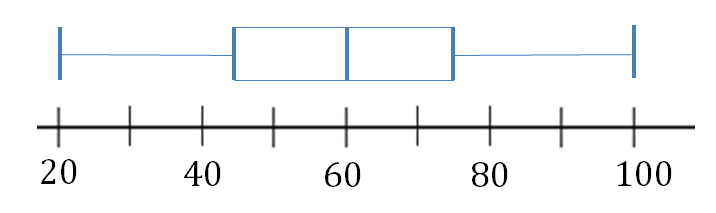
- Use the ogive below to draw a box-and-whisker plot:
- The ages of 28 people whose birthday coincides with that of one of their children are shown below.
[latex]\scriptsize \displaystyle \begin{align*}78;\text{ }53;\text{ }70;\text{ }97;\text{ }37;\text{ }68;\text{ }48;\text{ }35;\text{ }71;\text{ }63;\text{ }47;\text{ }60;\text{ }63;\text{ }58;\\74;\text{ }39;\text{ }67;\text{ }64;\text{ }42;\text{ }52;\text{ }38;\text{ }54;\text{ }60;\text{ }75;\text{ }69;\text{ }77;\text{ }65;\text{ }72\end{align*}[/latex]- Construct the frequency distribution showing cumulative frequency.
- Draw the ogive for the data.
- Estimate the median.
The full solutions are at the end of the unit.
Unit 2: Solutions
Exercise 2.1
- Construct a frequency distribution before drawing the cumulative frequency graph.
- .
Age intervals Frequency Cumulative frequency [latex]\scriptsize 0 \lt x\le 8[/latex] [latex]\scriptsize 6[/latex] [latex]\scriptsize 6[/latex] [latex]\scriptsize 8 \lt x\le 16[/latex] [latex]\scriptsize 1[/latex] [latex]\scriptsize 7[/latex] [latex]\scriptsize 16 \lt x\le 24[/latex] [latex]\scriptsize 3[/latex] [latex]\scriptsize 10[/latex] [latex]\scriptsize 24 \lt x\le 32[/latex] [latex]\scriptsize 1[/latex] [latex]\scriptsize 11[/latex] [latex]\scriptsize 32 \lt x\le 40[/latex] [latex]\scriptsize 4[/latex] [latex]\scriptsize 15[/latex] [latex]\scriptsize 40 \lt x\le 48[/latex] [latex]\scriptsize 2[/latex] [latex]\scriptsize 17[/latex] [latex]\scriptsize 48 \lt x\le 56[/latex] [latex]\scriptsize 1[/latex] [latex]\scriptsize 18[/latex] [latex]\scriptsize 56 \lt x\le 64[/latex] [latex]\scriptsize 2[/latex] [latex]\scriptsize 20[/latex] [latex]\scriptsize 64 \lt x\le 72[/latex] [latex]\scriptsize 1[/latex] [latex]\scriptsize 21[/latex] [latex]\scriptsize 72 \lt x\le 80[/latex] [latex]\scriptsize 3[/latex] [latex]\scriptsize 24[/latex] 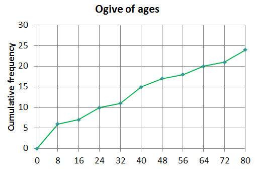
- Below [latex]\scriptsize 34[/latex]: as there are [latex]\scriptsize 24[/latex] values the median will be between positions [latex]\scriptsize 11[/latex] and [latex]\scriptsize 12[/latex]. Reading off the graph that gives us approximately [latex]\scriptsize 34[/latex].
- Below [latex]\scriptsize 24[/latex].
- .
- .
- [latex]\scriptsize 20[/latex] learners. Read off from the graph and subtract [latex]\scriptsize (35-15=20)[/latex].
- [latex]\scriptsize 15[/latex] learners. At least [latex]\scriptsize 70[/latex] means [latex]\scriptsize 70[/latex] or more, so subtract the number of learners at [latex]\scriptsize 70[/latex] from the number at [latex]\scriptsize 100[/latex] [latex]\scriptsize (50-35=15)[/latex].
- The median mark will be approximately [latex]\scriptsize 60\%[/latex].
Unit 2: Assessment
- .
- [latex]\scriptsize 120[/latex] observations in total.
- .
Intervals Frequency Cumulative frequency [latex]\scriptsize \displaystyle ~0 \lt x\le 10[/latex] [latex]\scriptsize \displaystyle 0[/latex] [latex]\scriptsize \displaystyle 0[/latex] [latex]\scriptsize \displaystyle 10 \lt x\le 20[/latex] [latex]\scriptsize \displaystyle 2[/latex] [latex]\scriptsize \displaystyle \mathbf{2}[/latex] [latex]\scriptsize \displaystyle 20 \lt x\le 30[/latex] [latex]\scriptsize \displaystyle 6[/latex] [latex]\scriptsize \displaystyle 8[/latex] [latex]\scriptsize \displaystyle 30 \lt x\le 40[/latex] [latex]\scriptsize \displaystyle 7[/latex] [latex]\scriptsize \displaystyle \mathbf{15}[/latex] [latex]\scriptsize \displaystyle 40 \lt x\le 50[/latex] [latex]\scriptsize \displaystyle 14[/latex] [latex]\scriptsize \displaystyle 29[/latex] [latex]\scriptsize \displaystyle 50 \lt x\le 60[/latex] [latex]\scriptsize \displaystyle 20[/latex] [latex]\scriptsize \displaystyle \mathbf{49}[/latex] [latex]\scriptsize \displaystyle 60 \lt x\le 70[/latex] [latex]\scriptsize \displaystyle 35[/latex] [latex]\scriptsize \displaystyle 84[/latex] [latex]\scriptsize \displaystyle 70 \lt x\le 80[/latex] [latex]\scriptsize \displaystyle 29[/latex] [latex]\scriptsize \displaystyle \mathbf{113}[/latex] [latex]\scriptsize \displaystyle 80 \lt x\le 90[/latex] [latex]\scriptsize \displaystyle 6[/latex] [latex]\scriptsize \displaystyle \mathbf{119}[/latex] [latex]\scriptsize \displaystyle 90 \lt x\le 100[/latex] [latex]\scriptsize \displaystyle 1[/latex] [latex]\scriptsize \displaystyle 120[/latex] - .
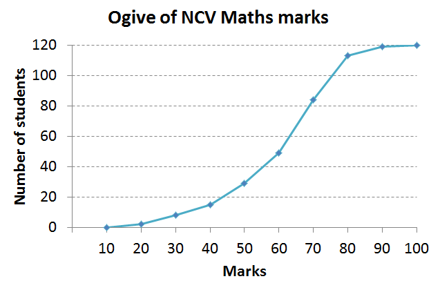
- There are [latex]\scriptsize 120[/latex] data values so the median will lie between position [latex]\scriptsize 60[/latex] and [latex]\scriptsize 61[/latex]. Looking at the cumulative frequency we see that the position of the median places it in the interval [latex]\scriptsize \displaystyle 60 \lt x\le 70[/latex].
- Reading off from the ogive, the median is approximately [latex]\scriptsize 63[/latex].
- .
[latex]\scriptsize \begin{align*}\text{Min}=20\\{{\text{Q}}_{1}}\approx 45\\{{\text{Q}}_{2}}\approx 60\\{{\text{Q}}_{3}}\approx 74\\\text{Max}=100\end{align*}[/latex]
- .
- .
Age intervals Frequency Cumulative frequency [latex]\scriptsize 34 \lt x\le 42[/latex] [latex]\scriptsize 5[/latex] [latex]\scriptsize 5[/latex] [latex]\scriptsize 42 \lt x\le 50[/latex] [latex]\scriptsize 2[/latex] [latex]\scriptsize 7[/latex] [latex]\scriptsize 50 \lt x\le 58[/latex] [latex]\scriptsize 4[/latex] [latex]\scriptsize 11[/latex] [latex]\scriptsize 58 \lt x\le 66[/latex] [latex]\scriptsize 6[/latex] [latex]\scriptsize 17[/latex] [latex]\scriptsize 66 \lt x\le 74[/latex] [latex]\scriptsize 7[/latex] [latex]\scriptsize 24[/latex] [latex]\scriptsize 74 \lt x\le 82[/latex] [latex]\scriptsize 3[/latex] [latex]\scriptsize 27[/latex] [latex]\scriptsize 82 \lt x\le 90[/latex] [latex]\scriptsize 0[/latex] [latex]\scriptsize 27[/latex] [latex]\scriptsize 90 \lt x\le 98[/latex] [latex]\scriptsize 1[/latex] [latex]\scriptsize 28[/latex] - .
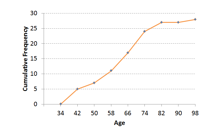
- Median age is approximately [latex]\scriptsize 63[/latex].
- .
Media Attributions
- Img 01_Ogive of ages Activity 2.1 © DHET is licensed under a CC BY (Attribution) license
- Activity 2.1 part E © DHET is licensed under a CC BY (Attribution) license
- Img 03_Example 2.1 © DHET is licensed under a CC BY (Attribution) license
- Example 2.2 © DHET is licensed under a CC BY (Attribution) license
- Exercise 2.1 Q2 © DHET is licensed under a CC BY (Attribution) license
- Assessment Q2 © DHET is licensed under a CC BY (Attribution) license
- Exercise 2.1 Q1a Answer © DHET is licensed under a CC BY (Attribution) license
- Assessment Q1c Ans © DHET is licensed under a CC BY (Attribution) license
- Assessment Q2 Ans © DHET is licensed under a CC BY (Attribution) license
- Assessment Q3b Ans © DHET is licensed under a CC BY (Attribution) license
