Unit outcomes

By the end of this unit you will be able to:

• Calculate the mean of grouped data using the formula [latex]\scriptsize \bar{x}=\displaystyle \frac{{\sum {{f}_{i}}{{x}_{i}}}}{n}[/latex].
• Calculate the median of grouped data using the formula [latex]\scriptsize \displaystyle {{\text{M}}_{e}}=l+\displaystyle \frac{{\left( {\displaystyle \frac{n}{2}-F} \right)}}{f}\times c[/latex].
• Calculate the modal value of grouped data using the formula [latex]\scriptsize {{M}_{o}}=l+\displaystyle \frac{{{{f}_{m}}-{{f}_{{m-1}}}}}{{2{{f}_{m}}-{{f}_{{m-1}}}-{{f}_{{m+1}}}}}\times c[/latex].

What you should know

Before you start this unit, make sure you can:

• Calculate central tendencies and dispersion of ungrouped data. To revise this topic you can review level 2, subject outcome 4.1.

Introduction

When only grouped data is available, we do not know the individual data values; we only know the intervals and interval frequencies, therefore we cannot compute exact measures of central tendency and dispersion for the data set. For grouped data we calculate estimated measures of central tendency and dispersion.

Take note!

Measures of central tendency or averages are single numbers that provide summary information about an entire set of data, without listing every single data value.

Measures of dispersion provide information on how spread out the data are around the centre values.

Measures of central tendency for grouped data

There are three main measures of central tendency: the mean, the median and the mode. In the following activity we learn how to find the mean, median and mode for grouped data using special formulae.

Activity 4.1: Calculate the mean, median and mode for grouped data

Time required: 30 minutes

What you need:

• a pen
• paper
• a calculator

What to do:

Answer the following questions and show all the necessary steps.

A survey was conducted among [latex]\scriptsize \displaystyle 50[/latex] recyclers. The mass of the waste each of them recycled in a month was recorded in the frequency table below.

Mass of recycling (in kg)	Midpoint of interval	Frequency	Midpoint [latex]\scriptsize \times[/latex] frequency
[latex]\scriptsize 40 \lt m\le 45[/latex]	[latex]\scriptsize \displaystyle \frac{{40+45}}{2}=42.5[/latex]	[latex]\scriptsize 7[/latex]	[latex]\scriptsize 7\times 42.5=297.5[/latex]
[latex]\scriptsize 45 \lt m\le 50[/latex]		[latex]\scriptsize 10[/latex]
[latex]\scriptsize 50 \lt m\le 55[/latex]		[latex]\scriptsize \displaystyle 15[/latex]
[latex]\scriptsize 55vm\le 60[/latex]		[latex]\scriptsize \displaystyle 12[/latex]
[latex]\scriptsize 60 \lt m\le 65[/latex]		[latex]\scriptsize \displaystyle 6[/latex]
	Total	[latex]\scriptsize \displaystyle 50[/latex]	[latex]\scriptsize \displaystyle 2\text{ }625[/latex]

1. Copy and complete the table.
2. Find the estimated mean using the formula [latex]\scriptsize \bar{x}=\displaystyle \frac{{\sum {{f}_{i}}{{x}_{i}}}}{n}[/latex], (where [latex]\scriptsize {{f}_{i}}{{x}_{i}}[/latex]is the product of the class or interval midpoint and the frequency).
3. Why do we call it the estimated mean when working with grouped data?
4. What is the modal class interval of the data?
5. Use the following formula to calculate the mode: [latex]\scriptsize {{M}_{o}}=l+\displaystyle \frac{{{{f}_{m}}-{{f}_{{m-1}}}}}{{2{{f}_{m}}-{{f}_{{m-1}}}-{{f}_{{m+1}}}}}\times c[/latex] (where [latex]\scriptsize l[/latex] is the lower limit of the modal class, [latex]\scriptsize c[/latex] is the class width,[latex]\scriptsize {{f}_{m}}[/latex] is the frequency of the modal class, [latex]\scriptsize {{f}_{{m-1}}}[/latex] is the frequency of the class before the modal class and [latex]\scriptsize {{f}_{{m+1}}}[/latex] is the frequency of the class after the modal class).
6. In which class interval will you find the median?
7. Use the following formula to calculate the median: [latex]\scriptsize \displaystyle {{\text{M}}_{e}}=l+\displaystyle \frac{{\left( {\displaystyle \frac{n}{2}-F} \right)}}{f}\times c[/latex] (where [latex]\scriptsize l[/latex] is the lower limit of the median class, [latex]\scriptsize n[/latex] is the number of observations,[latex]\scriptsize \displaystyle F[/latex] is the cumulative frequency of the class before the median class,[latex]\scriptsize \displaystyle f[/latex] is the frequency of the median class and [latex]\scriptsize c[/latex] is the class width).

What did you find?

1. Below is the completed table.
   

   Mass of recycling (in kg)	Midpoint of interval	Frequency	Midpoint [latex]\scriptsize \times[/latex] frequency
   [latex]\scriptsize 40 \lt m\le 45[/latex]	[latex]\scriptsize \displaystyle \frac{{40+45}}{2}=42.5[/latex]	[latex]\scriptsize 7[/latex]	[latex]\scriptsize 7\times 42.5=297.5[/latex]
   [latex]\scriptsize 45 \lt m\le 50[/latex]	[latex]\scriptsize 47.5[/latex]	[latex]\scriptsize 10[/latex]	[latex]\scriptsize \displaystyle 10\left( {47.5} \right)=475[/latex]
   [latex]\scriptsize 50 \lt m\le 55[/latex]	[latex]\scriptsize 52.5[/latex]	[latex]\scriptsize \displaystyle 15[/latex]	[latex]\scriptsize \displaystyle 15\left( {52.5} \right)=787.5[/latex]
   [latex]\scriptsize 55 \lt m\le 60[/latex]	[latex]\scriptsize 57.5[/latex]	[latex]\scriptsize \displaystyle 12[/latex]	[latex]\scriptsize \displaystyle 12\left( {57.5} \right)=690[/latex]
   [latex]\scriptsize 60 \lt m\le 65[/latex]	[latex]\scriptsize 62.5[/latex]	[latex]\scriptsize \displaystyle 6[/latex]	[latex]\scriptsize \displaystyle 6\left( {62.5} \right)=375[/latex]
   	Total	[latex]\scriptsize \displaystyle 50[/latex]	[latex]\scriptsize \displaystyle 2\text{ }625[/latex]

2. The estimated mean is calculated as:
   [latex]\scriptsize \begin{align*}\bar{x}&=\displaystyle \frac{{7\left( {42.5} \right)+10\left( {47.5} \right)+15\left( {52.5} \right)+12\left( {57.5} \right)+6\left( {62.5} \right)}}{{50}}\\&=\displaystyle \frac{{2\text{ }625}}{{50}}\\&=52.5\text{ kg}\end{align*}[/latex]
3. We are working with grouped data rather than the original ungrouped data hence some information has been lost when the grouped intervals were created. So the best we can do is approximate the mean.
4. The modal class is the interval with the highest number of data values (frequency). Therefore, the modal interval is [latex]\scriptsize \displaystyle 50 \lt m\le 55[/latex], as the highest frequency is recorded in that interval.
5. We can estimate the mode using the formula:
   [latex]\scriptsize \begin{align*}{{M}_{o}}&=50+\displaystyle \frac{{15-10}}{{2(15)-10-12}}\times 5\\&=50+\displaystyle \frac{{25}}{8}\\&=53.125\text{ kg}\end{align*}[/latex]
6. The median will be found in the central interval when the intervals are arranged in order. Since there are [latex]\scriptsize \displaystyle 50[/latex] values altogether the median will be found between the [latex]\scriptsize \displaystyle 25\text{th}[/latex] and [latex]\scriptsize \displaystyle 26\text{th}[/latex] values. By adding the frequencies of the intervals, we see that the median will be located in the [latex]\scriptsize \displaystyle 50 \lt m\le 55[/latex] interval.
7. .
   [latex]\scriptsize \displaystyle \begin{align*}{{\text{M}}_{e}}&=50+\displaystyle \frac{{\left( {\displaystyle \frac{{50}}{2}-17} \right)}}{{15}}\times 5\\&=50+\displaystyle \frac{8}{3}\\&=52.67\end{align*}[/latex]

Below are the formulae you will use to calculate the estimated mean, median and mode for grouped data.

Example 4.1

A survey was conducted among [latex]\scriptsize \displaystyle 50[/latex] recyclers. The mass of the waste each of them recycled in a month was recorded in the frequency table below.

Mass of recycling (in kg)	Midpoint of interval	Frequency	Midpoint [latex]\scriptsize \times[/latex] frequency
[latex]\scriptsize 40 \lt m\le 45[/latex]	[latex]\scriptsize \displaystyle \frac{{40+45}}{2}=42.5[/latex]	[latex]\scriptsize 7[/latex]	[latex]\scriptsize 7\times 42.5=297.5[/latex]
[latex]\scriptsize 45 \lt m\le 50[/latex]	[latex]\scriptsize 47.5[/latex]	[latex]\scriptsize 10[/latex]	[latex]\scriptsize \displaystyle 10\left( {47.5} \right)=475[/latex]
[latex]\scriptsize 50 \lt m\le 55[/latex]	[latex]\scriptsize 52.5[/latex]	[latex]\scriptsize \displaystyle 15[/latex]	[latex]\scriptsize \displaystyle 15\left( {52.5} \right)=787.5[/latex]
[latex]\scriptsize 55 \lt m\le 60[/latex]	[latex]\scriptsize 57.5[/latex]	[latex]\scriptsize \displaystyle 12[/latex]	[latex]\scriptsize \displaystyle 12\left( {57.5} \right)=690[/latex]
[latex]\scriptsize 60 \lt m\le 65[/latex]	[latex]\scriptsize 62.5[/latex]	[latex]\scriptsize \displaystyle 6[/latex]	[latex]\scriptsize \displaystyle 6\left( {62.5} \right)=375[/latex]
	Total	[latex]\scriptsize \displaystyle 50[/latex]	[latex]\scriptsize \displaystyle 2\text{ }625[/latex]

Use a calculator to find the mean for the data.

Solution

It is very rare in real life applications that statistics will be computed by hand. In this example we will use the Casio fx-82ZA calculator to find the mean for the grouped data from Activity 4.1. Make sure that you consult your calculator manual for steps specific to your calculator.

Step 1: As you are working with grouped data we need to tell the calculator that we are using frequencies. To do that: Press SHIFT MODE (SET UP). Scroll down using the arrows and Select 3: STAT

The calculator display says frequency 1: On or 2: Off. Select 1: On

Step 2: Press MODE and 2: STAT then Select 1: 1-VAR

Step 3: Enter the class midpoint under the ‘[latex]\scriptsize X[/latex]’ column and press [latex]\scriptsize =[/latex]. Next enter the corresponding frequency under the FREQ column and press [latex]\scriptsize =[/latex]. You can use the arrows to scroll and correct any mistakes.

After you have finished entering the data, press AC. Don’t panic when the values disappear! The data entering screen will disappear but the data has been stored and can be brought back if required.

Step 4: To find the summary statistics including the mean press SHIFT ‘1’ (STAT).

Press 4: VAR: all the summary statistics will be found here.

Press 2: [latex]\scriptsize \displaystyle ~\overline{x}=[/latex] for the estimated mean. Note: your answer should be the same as the value [latex]\scriptsize \displaystyle \left( {52.5\text{ kg}} \right)[/latex] calculated manually in Activity 4.1. If not then you have made a mistake.

We will use these same calculator steps to find the variance and standard deviation for data in Maths Level 4 so make sure you understand how to use your calculator.

Exercise 4.1

1. The following data shows the number of hours over the weekend that teenagers play video games.
   

   Hours spent on video games	Frequency
   [latex]\scriptsize (0;3.5][/latex]	[latex]\scriptsize 3[/latex]
   [latex]\scriptsize (3.5;7.5][/latex]	[latex]\scriptsize 7[/latex]
   [latex]\scriptsize \displaystyle (7.5;11.5][/latex]	[latex]\scriptsize 12[/latex]
   [latex]\scriptsize (11.5;15.5][/latex]	[latex]\scriptsize 7[/latex]
   [latex]\scriptsize (15.5;19.5][/latex]	[latex]\scriptsize 9[/latex]

   What is the best estimate for the mean number of hours spent playing video games?

2. In a traffic survey a random sample of [latex]\scriptsize \displaystyle 50[/latex] motorists were asked what distance they drove to work daily. The results of the survey are shown in kilometres in the table below.
   

   Distance	[latex]\scriptsize 0 \lt d\le 10[/latex]	[latex]\scriptsize 10 \lt d\le 20[/latex]	[latex]\scriptsize 20 \lt d\le 30[/latex]	[latex]\scriptsize 30 \lt d\le 40[/latex]	[latex]\scriptsize 40 \lt d\le 50[/latex]
   Frequency	[latex]\scriptsize 9[/latex]	[latex]\scriptsize 17[/latex]	[latex]\scriptsize 15[/latex]	[latex]\scriptsize 5[/latex]	[latex]\scriptsize 4[/latex]
   Midpoint [latex]\scriptsize {{x}_{i}}[/latex]
   [latex]\scriptsize {{f}_{i}}\times {{x}_{i}}[/latex]

   1. Copy and complete the table.
   2. Calculate the mean distance.
   3. Calculate the mode.
   4. Calculate the median distance.
   5. Draw the ogive for the data using cumulative frequencies.

The full solutions are at the end of the unit.

Measures of dispersion

Variation is present in any set of data. For example, a [latex]\scriptsize 300\text{ ml}[/latex] can of cooldrink may contain slightly more or slightly less than [latex]\scriptsize 300\text{ ml}[/latex]. Manufacturers regularly run tests to determine if the amount of beverage in a can falls within the desired range.

To find out how scattered the data values are from the mean we must calculate the measures of variability, called measures of dispersion.

The range, interquartile range and standard deviation are the three commonly used measures of dispersion.

Be aware that when you collect data, your data may vary somewhat from the data someone else is collecting for the same purpose. This is completely natural. However, if two or more of you are collecting the same data and get very different results, it is time to re-evaluate the data methods and accuracy.

Take note!

Measures of dispersion show how much the data vary from the average value of a data set.

Interquartile range

The interquartile range (IQR) is a number that shows the spread of the middle half or the middle [latex]\scriptsize \displaystyle 50\%[/latex] of the data. It is the difference between the third quartile [latex]\scriptsize \displaystyle \left( {{{\text{Q}}_{3}}} \right)[/latex] and the first quartile [latex]\scriptsize \displaystyle \left( {{{\text{Q}}_{1}}} \right)[/latex]. The IQR is a good measure of the spread of data as it is not affected by outliers.

Example 4.2

Below is the ogive of the ages of people attending a public reading by an author at a library.

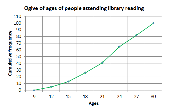
1. Find [latex]\scriptsize {{\text{Q}}_{3}}[/latex].
2. What age are [latex]\scriptsize 75\%[/latex] of the people younger than?
3. Find [latex]\scriptsize {{\text{Q}}_{1}}[/latex] .
4. [latex]\scriptsize 25\%[/latex] of the people are less than _____ years old.
5. Find the IQR. What does this value tell us?

Solution

We can read the answers from the graph shown below.

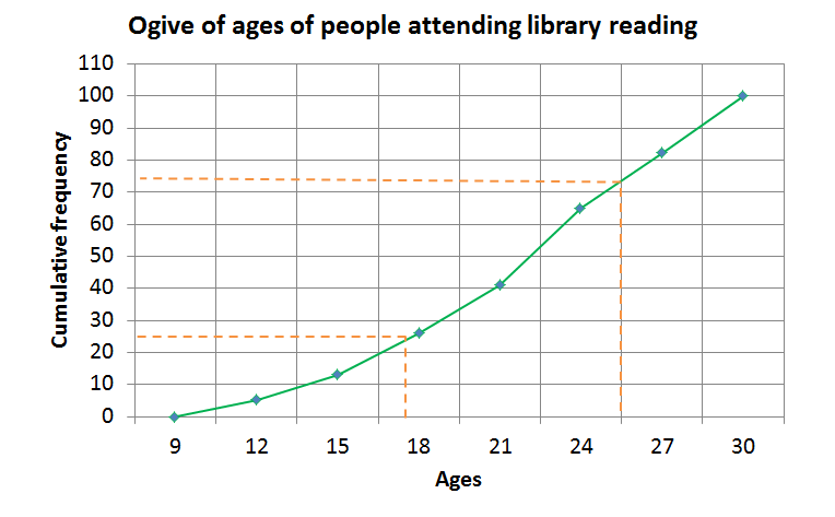
1. There are [latex]\scriptsize 100[/latex] people attending the reading therefore, [latex]\scriptsize {{\text{Q}}_{3}}[/latex] is in position [latex]\scriptsize 75[/latex] [latex]\scriptsize (\displaystyle \frac{3}{4}\times 100=75)[/latex]. We can read the value from the graph, [latex]\scriptsize {{\text{Q}}_{3}}\approx 25[/latex].
2. [latex]\scriptsize {{\text{Q}}_{3}}[/latex] is the value that [latex]\scriptsize 75\%[/latex] of the data values are less than. Therefore, [latex]\scriptsize 75\%[/latex] of the people are younger than [latex]\scriptsize 25[/latex].
3. [latex]\scriptsize {{\text{Q}}_{1}}[/latex] is in position [latex]\scriptsize 25[/latex] [latex]\scriptsize (\displaystyle \frac{1}{4}\times 100=25)[/latex], from the graph this corresponds to approximately [latex]\scriptsize 17[/latex].
4. [latex]\scriptsize 25\%[/latex] of the people are less than [latex]\scriptsize 17[/latex] years old.
5. [latex]\scriptsize \text{IQR}=25-17=8[/latex]
   The IQR tells us that the middle [latex]\scriptsize 50\%[/latex] of ages vary by about [latex]\scriptsize 8[/latex] years. We can also tell that [latex]\scriptsize 50\%[/latex] of the people are aged between [latex]\scriptsize 17[/latex] and [latex]\scriptsize 25[/latex] years old.

The interquartile range is very useful when you compare different sets of data. A larger IQR means the data are more spread out (varied) and a lower IQR shows less variability.

Example 4.3

We need to compare two sets of maths marks for Class A and Class B. We are given the following information.

Class A:

[latex]\scriptsize \text{Mean}=\text{median}=\text{mode}=55\%[/latex]

[latex]\scriptsize \text{IQR}=45\%[/latex]

[latex]\scriptsize \text{Range}=75\%[/latex]

Class B:

[latex]\scriptsize \text{Mean}=\text{median}=\text{mode}=55\%[/latex]

[latex]\scriptsize \text{IQR}=35\%[/latex]

[latex]\scriptsize \text{Range}=80\%[/latex]

Which class performed better in the test?

Solution

Both data sets have the same mean, median and mode but the data values may be very different. So by just focusing on the measures of central tendency you may arrive at the incorrect conclusion that both classes performed the same.

The range of Class B is higher than the range of Class A but the range is easily affected by outliers so it is not the best measure of variability of the data.

The IQR for Class B is lower than the IQR for Class A. This means there is less variability in the middle [latex]\scriptsize 50\%[/latex] of the marks for Class B, therefore, Class B performed better than Class A.

Exercise 4.2

The marks (as a percentage) obtained in an NCV Maths Level 3 examination are shown in the ogive.

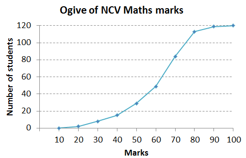
1. How many learners’ marks were recorded?
2. [latex]\scriptsize 75\%[/latex] of learners scored less than what mark?
3. [latex]\scriptsize 25\%[/latex] of learners scored less than what mark?
4. [latex]\scriptsize 75\%[/latex] of learners scored more than what mark?
5. Find the interquartile range.

The full solutions are at the end of the unit.

Summary

In this unit you have learnt the following:

• How to find the mean, median and mode for grouped data.
• How to use the ogive to find the interquartile range.
• How to interpret the interquartile range.

Unit 4: Assessment

Suggested time to complete: 30 minutes

1. The following table shows the amount (in Rand) that [latex]\scriptsize 50[/latex] families, who live in apartments, spent on prepaid electricity.
   

   Electricity cost (Rand amount)	Number of families
   [latex]\scriptsize 450 \lt \text{R}\le 600[/latex]	[latex]\scriptsize \displaystyle 4[/latex]
   [latex]\scriptsize 600 \lt \text{R}\le 750[/latex]	[latex]\scriptsize \displaystyle 12[/latex]
   [latex]\scriptsize 750 \lt \text{R}\le 900[/latex]	[latex]\scriptsize \displaystyle 16[/latex]
   [latex]\scriptsize 900 \lt \text{R}\le 1050[/latex]	[latex]\scriptsize \displaystyle 10[/latex]
   [latex]\scriptsize 1050 \lt \text{R}\le 1150[/latex]	[latex]\scriptsize \displaystyle 8[/latex]

   1. Complete the frequency table.
      

      Electricity cost (Rand amount)	Class midpoint	Number of families	Frequency [latex]\scriptsize \times[/latex] class midpoint
      [latex]\scriptsize 450 \lt \text{R}\le 600[/latex]		[latex]\scriptsize \displaystyle 4[/latex]
      [latex]\scriptsize 600 \lt \text{R}\le 750[/latex]		[latex]\scriptsize \displaystyle 12[/latex]
      [latex]\scriptsize 750 \lt \text{R}\le 900[/latex]		[latex]\scriptsize \displaystyle 16[/latex]
      [latex]\scriptsize 900 \lt \text{R}\le 1050[/latex]		[latex]\scriptsize \displaystyle 10[/latex]
      [latex]\scriptsize 1050 \lt \text{R}\le 1150[/latex]		[latex]\scriptsize \displaystyle 8[/latex]

   2. What was the average amount spent on electricity?
   3. Calculate the median amount.
   4. Compare the mean amount to the median and comment on the skewness of the data.
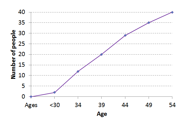
2. The table below shows the ages of people attending a local gym on one particular day. Study the table and answer the questions that follow.
   

   Ages	Frequency	Cumulative frequency
   [latex]\scriptsize \lt 30[/latex]	[latex]\scriptsize 2[/latex]	[latex]\scriptsize 2[/latex]
   [latex]\scriptsize 30-34[/latex]	[latex]\scriptsize 10[/latex]	[latex]\scriptsize 12[/latex]
   [latex]\scriptsize 35-39[/latex]	[latex]\scriptsize 8[/latex]	[latex]\scriptsize 20[/latex]
   [latex]\scriptsize 40-44[/latex]	[latex]\scriptsize 9[/latex]	[latex]\scriptsize 29[/latex]
   [latex]\scriptsize 45-49[/latex]	[latex]\scriptsize 6[/latex]	[latex]\scriptsize 35[/latex]
   [latex]\scriptsize 50-54[/latex]	[latex]\scriptsize 5[/latex]	[latex]\scriptsize 40[/latex]

   1. Sketch the ogive curve of the data.
   2. Use the ogive curve to find the interquartile range by first estimating the values for the first and third quartiles.

The full solutions are at the end of the unit.

Unit 4: Solutions

Exercise 4.1

1. Find the class midpoint and frequency multiplied by class midpoint first.
   

   Hours spent on video games	Class midpoint[latex]\scriptsize {{x}_{i}}[/latex]	Frequency	[latex]\scriptsize {{f}_{i}}\times {{x}_{i}}[/latex]
   [latex]\scriptsize (0;3.5][/latex]	[latex]\scriptsize 1.75[/latex]	[latex]\scriptsize 3[/latex]	[latex]\scriptsize 1.75\times 3=5.25[/latex]
   [latex]\scriptsize (3.5;7.5][/latex]	[latex]\scriptsize 5.5[/latex]	[latex]\scriptsize 7[/latex]	[latex]\scriptsize 5.5\times 7=38.5[/latex]
   [latex]\scriptsize \displaystyle (7.5;11.5][/latex]	[latex]\scriptsize 9.5[/latex]	[latex]\scriptsize 12[/latex]	[latex]\scriptsize 9.5\times 12=114[/latex]
   [latex]\scriptsize (11.5;15.5][/latex]	[latex]\scriptsize 13.5[/latex]	[latex]\scriptsize 7[/latex]	[latex]\scriptsize 13.5\times 7=94.5[/latex]
   [latex]\scriptsize (15.5;19.5][/latex]	[latex]\scriptsize 9[/latex]	[latex]\scriptsize 9[/latex]	[latex]\scriptsize 17.5\times 9=157.5[/latex]
   	Total	[latex]\scriptsize 38[/latex]	[latex]\scriptsize \sum{{{{f}_{i}}\times {{x}_{i}}=409.75}}[/latex]

   [latex]\scriptsize \displaystyle \begin{align*}\bar{x}&=\displaystyle \frac{{\sum {{f}_{i}}{{x}_{i}}}}{n}\\&=\displaystyle \frac{{409.75}}{{38}}\\&=10.78\text{ hours}\end{align*}[/latex]

2. .
   1. .
      

      Distance	[latex]\scriptsize 0 \lt d\le 10[/latex]	[latex]\scriptsize 10 \lt d\le 20[/latex]	[latex]\scriptsize 20 \lt d\le 30[/latex]	[latex]\scriptsize 30 \lt d\le 40[/latex]	[latex]\scriptsize 40 \lt d\le 50[/latex]
      Frequency	[latex]\scriptsize 9[/latex]	[latex]\scriptsize 17[/latex]	[latex]\scriptsize 15[/latex]	[latex]\scriptsize 5[/latex]	[latex]\scriptsize 4[/latex]
      Midpoint [latex]\scriptsize {{x}_{i}}[/latex]	[latex]\scriptsize 5[/latex]	[latex]\scriptsize 15[/latex]	[latex]\scriptsize 25[/latex]	[latex]\scriptsize 35[/latex]	[latex]\scriptsize 45[/latex]
      [latex]\scriptsize {{f}_{i}}\times {{x}_{i}}[/latex]	[latex]\scriptsize 45[/latex]	[latex]\scriptsize 255[/latex]	[latex]\scriptsize 375[/latex]	[latex]\scriptsize 175[/latex]	[latex]\scriptsize 180[/latex]

   2. The mean distance is [latex]\scriptsize 20.6\text{ km}[/latex].
   3. The modal interval is [latex]\scriptsize 10 \lt d\le 20[/latex] with a frequency of [latex]\scriptsize 17[/latex].
      [latex]\scriptsize \begin{align*}{{M}_{o}}&=l+\displaystyle \frac{{{{f}_{m}}-{{f}_{{m-1}}}}}{{2{{f}_{m}}-{{f}_{{m-1}}}-{{f}_{{m+1}}}}}\times c\\&=10+\displaystyle \frac{{17-9}}{{2(17)-9-15}}\times 10\\&=18\text{ km}\end{align*}[/latex]
   4. Median:
      [latex]\scriptsize \displaystyle \begin{align*}{{\text{M}}_{e}}&=l+\displaystyle \frac{{\left( {\displaystyle \frac{n}{2}-F} \right)}}{f}\times c\\&=10+\displaystyle \frac{{25-9}}{{17}}\times 10\\&=19.4\text{ km}\end{align*}[/latex]
   5. Find the cumulative frequencies first and then plot against the distance to give the ogive below.
      

Back to Exercise 4.1

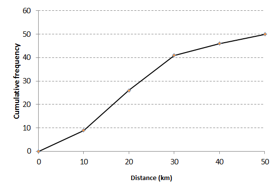
Exercise 4.2

1. There are [latex]\scriptsize 120[/latex] observations.

The ogive below is used to answer questions 2 to 5.

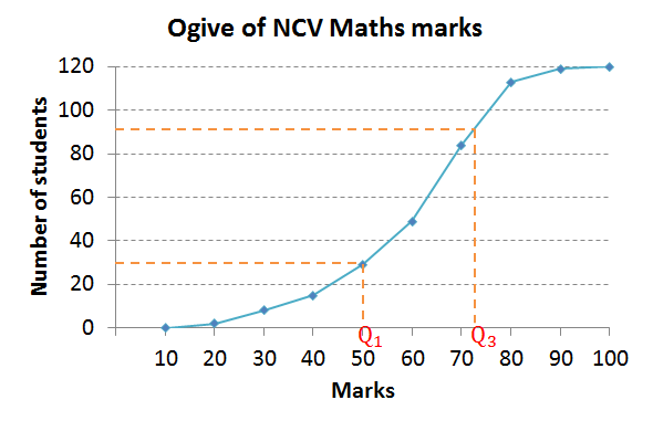
2. [latex]\scriptsize 0.75\times 120=90[/latex] so we must find the third quartile from position [latex]\scriptsize 90[/latex] on the vertical axis of ogive as shown in the graph. We see that [latex]\scriptsize 75\%[/latex] of learners got less than [latex]\scriptsize 72\%[/latex].
3. [latex]\scriptsize 0.25\times 120=30[/latex] so we must look for [latex]\scriptsize 30[/latex] on the y-axis and draw a horizontal line until we reach the graph and then read off the marks from the x-axis. We see that [latex]\scriptsize 25\%[/latex] of learners scored less than [latex]\scriptsize 50\%[/latex].
4. Since [latex]\scriptsize 25\%[/latex] of learners scored less than [latex]\scriptsize 50\%[/latex] this means [latex]\scriptsize 75\%[/latex] of learners scored more than [latex]\scriptsize 50\%[/latex].
5. .
   [latex]\scriptsize \begin{align*}\text{IQR}&=72\%-50\%\\&=22\%\end{align*}[/latex]

Back to Exercise 4.2

Unit 4: Assessment

1. .
   1. .
      

      Electricity cost (Rand amount)	Class midpoint	Number of families	Frequency [latex]\scriptsize \times[/latex] class midpoint
      [latex]\scriptsize 450 \lt \text{R}\le 600[/latex]	[latex]\scriptsize \displaystyle 525[/latex]	[latex]\scriptsize \displaystyle 4[/latex]	[latex]\scriptsize \displaystyle 2\text{ }100[/latex]
      [latex]\scriptsize 600 \lt \text{R}\le 750[/latex]	[latex]\scriptsize \displaystyle 675[/latex]	[latex]\scriptsize \displaystyle 12[/latex]	[latex]\scriptsize \displaystyle 8\text{ }100[/latex]
      [latex]\scriptsize 750 \lt \text{R}\le 900[/latex]	[latex]\scriptsize \displaystyle 825[/latex]	[latex]\scriptsize \displaystyle 16[/latex]	[latex]\scriptsize \displaystyle 13\text{ }200[/latex]
      [latex]\scriptsize 900 \lt \text{R}\le 1050[/latex]	[latex]\scriptsize \displaystyle 975[/latex]	[latex]\scriptsize \displaystyle 10[/latex]	[latex]\scriptsize \displaystyle 9\text{ }750[/latex]
      [latex]\scriptsize 1050 \lt \text{R}\le 1150[/latex]	[latex]\scriptsize \displaystyle 1\text{ }100[/latex]	[latex]\scriptsize \displaystyle 8[/latex]	[latex]\scriptsize \displaystyle 8\text{ }800[/latex]
      	Total	[latex]\scriptsize \displaystyle 50[/latex]	[latex]\scriptsize \displaystyle 41\text{ }950[/latex]

       

   2. Average amount spent:
      [latex]\scriptsize \begin{align*}\bar{x}&=\displaystyle \frac{{\sum {{f}_{i}}{{x}_{i}}}}{n}\\&=\displaystyle \frac{{41\text{ }950}}{{50}}\\&=\text{ R }839\end{align*}[/latex]
   3. The median will be found in the interval [latex]\scriptsize \displaystyle 750 \lt \text{R}\le 900[/latex].
      [latex]\scriptsize \displaystyle \begin{align*}{{\text{M}}_{e}}&=l+\displaystyle \frac{{\left( {\displaystyle \frac{n}{2}-F} \right)}}{f}\times c\\&=750+\displaystyle \frac{{25-16}}{{16}}\times 150\\&=\text{R}834.38\end{align*}[/latex]
   4. mean [latex]\scriptsize \gt[/latex] median by a small amount so the data will be slightly skewed to the right.
2. .
   1. .
      
   2. .
      Use the graph below to answer this part of the question by reading off from the graph.
      
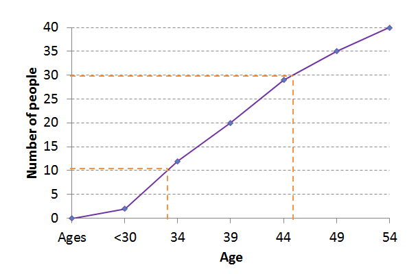
      [latex]\scriptsize {{\text{Q}}_{1}}\approx 33[/latex]
      [latex]\scriptsize {{\text{Q}}_{3}}=45[/latex]
      [latex]\scriptsize \begin{align*}\text{IQR}&=45-33\\&=12\end{align*}[/latex]

Back to Unit 4: Assessment