Data handling: Calculate, represent and interpret measures of central tendency and dispersion in univariate numerical ungrouped data
Unit 2: The five-number summary and box-and-whisker diagram
Natashia Bearam-Edmunds
Unit outcomes
By the end of this unit you will be able to:
- Combine measures of central tendency and dispersion to work out the five-number summary.
- Construct the box-and-whisker plot.
- Interpret the box-and-whisker plot.
What you should know
Before you start this unit, make sure you can:
- Calculate central tendencies and dispersion of data and represent data effectively. Revise the following level 2, topic 4 units on data handling:
- Subject outcome 4.1, unit 1: data collecting.
- Subject outcome 4.1, unit 2: measures of central tendency of ungrouped data.
- Subject outcome 4.1, unit 3: measures of dispersion of ungrouped data.
- Subject outcome 4.2, unit 1: data representation.
- Subject outcome 4.2, unit 2: bar graphs and histograms.
- Subject outcome 4.2, unit 3: frequency polygon and line graphs.
Introduction
To have a good understanding of data, and for a better overall picture of what it’s telling us, we must combine the measures of central tendency with the measures of dispersion. The five-number summary combines a measure of central tendency (the median) with measures of dispersion, the range and the inter-quartile range. A box-and-whisker-plot or box plot is a visual display of the five-number summary that helps us see the trends in data.
Box plots show how the quartiles divide the data into sections where each section contains approximately [latex]\scriptsize \displaystyle 25\%[/latex] of the data in that set. The five-number summary is listed in the following order: minimum, first quartile, median, third quartile and maximum.
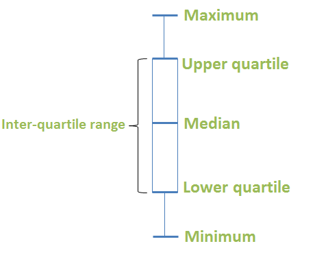
Minimum value: The lowest value in a data set.
Lower quartile: [latex]\scriptsize \displaystyle (~{{\text{Q}}_{1}})[/latex]: The median of the lower half of an ordered data set.
Median: [latex]\scriptsize \displaystyle (~{{\text{Q}}_{2}})[/latex]: The median is the middle value of an ordered data set.
Upper quartile: [latex]\scriptsize \displaystyle (~{{\text{Q}}_{3}})[/latex]: The median of the upper half of an ordered data set.
Maximum value: The highest value in a data set.
Work through Activity 2.1 to get a better understanding of how to represent the five-number summary using a box-and-whisker diagram.
Activity 2.1: Constructing a box plot
Time required: 15 minutes
What you need:
- a pen and paper
What to do:
The following data set shows the maths marks of eight learners:
[latex]\scriptsize \displaystyle 62;\text{ }56;\text{ }71;\text{ }78;\text{ }89;\text{ }92;\text{ }86;\text{ }74[/latex]
- Rewrite the data set in ascending order.
- Find the maximum and minimum marks.
- Calculate the median mark.
- Calculate the lower and upper quartiles.
- Write down the values for the five-number summary.
- Use a number line to show the information you have calculated. Indicate where the answers to question 5 are located. Draw a box around the IQR and join it to the minimum and maximum values.
- Indicate if there are any outliers in this data set.
What did you find?
- The values arranged from lowest to highest: [latex]\scriptsize \displaystyle 56;\text{ }62;\text{ }71;\text{ }74;\text{ }78;\text{ }86;\text{ }89;\text{ }92[/latex]
- The maximum mark is [latex]\scriptsize \displaystyle 92[/latex] and the minimum mark is [latex]\scriptsize \displaystyle 56[/latex].
- The median, also called the second quartile, will lie between the [latex]\scriptsize \displaystyle 4\text{th}[/latex] and [latex]\scriptsize \displaystyle 5\text{th}[/latex] values. [latex]\scriptsize \text{M}=\displaystyle \frac{{74+78}}{2}=76[/latex].
- .
[latex]\scriptsize \begin{align*}{{\text{Q}}_{1}}&=\displaystyle \frac{{62+71}}{2}\\&=66.5\\{{\text{Q}}_{3}}&=\displaystyle \frac{{86+89}}{2}\\&=87.5\end{align*}[/latex] - Minimum [latex]\scriptsize \displaystyle =56[/latex]
First quartile [latex]\scriptsize \displaystyle =66.5[/latex]
Median [latex]\scriptsize \displaystyle =76[/latex]
Third quartile [latex]\scriptsize \displaystyle =87.5[/latex]
Maximum [latex]\scriptsize \displaystyle =92[/latex] - Mark off the points above the number line and draw a box around the IQR, join it to the minimum and maximum values to get the box-and-whisker plot from the number line.
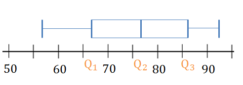
The box shows the distance between [latex]\scriptsize {{\text{Q}}_{1}}[/latex] and [latex]\scriptsize {{\text{Q}}_{3}}[/latex] (IQR). A line inside the box shows the median. The lines extending outside the box (the whiskers) show where the minimum and maximum values are located. Note: this graph can be drawn vertically too. - To check for outliers use the [latex]\scriptsize \text{1}\text{.5}\times \text{IQR}[/latex] rule.
[latex]\scriptsize \begin{align*}\text{IQR}&=87.5-66.5\\&=21\\1.5\times \text{IQR}&=1.5(21)\\&=31.5\\{{\text{Q}}_{1}}-31.5&=35\\{{\text{Q}}_{3}}+31.5&=119\end{align*}[/latex]
There are no outliers in this data set.
Take note!
To identify outliers, upper and lower fences are used to set limits of data values. The formula for the upper fence is [latex]\scriptsize {{\text{Q}}_{3}}+1.5\times \text{IQR}[/latex] and the formula for the lower fence is [latex]\scriptsize {{\text{Q}}_{1}}-1.5\times \text{IQR}[/latex] where IQR is the interquartile range. The lower fence is the lower limit and the upper fence is the upper limit. Any value outside of these fences is considered an outlier.
The diagram below shows the main parts of a box and whisker plot.
Take note!
It is important to start a box plot with a scaled number line. Otherwise the box plot may not be useful.
Example 2.1
Douglas works as a telesales person. He keeps a record of the number of sales he makes each month. The data below show how much he sells each month.
[latex]\scriptsize \displaystyle \{49;\text{ 70};\text{ }22;\text{ }35;\text{ 68};\text{ }45;\text{ }60;\text{ }48;\text{ }19;\text{ 120};\text{ }43;\text{ }12\}[/latex]
- Calculate his median number of sales.
- Give the five-number summary.
- Draw a box-and-whisker plot of the sales. Find the upper and lower fences and show any outliers on your box-and-whisker plot.
Solution
- Order the data: [latex]\scriptsize \displaystyle \{12;\text{ }19;\text{ }22;\text{ }35;\text{ }43;\text{ }45;\text{ }48;\text{ }49;\text{ }60;\text{ 68};\text{ 70};\text{ 120}\}\text{ }[/latex]
[latex]\scriptsize \begin{align*}\text{M}&=\displaystyle \frac{{45+48}}{2}\\&=46.5\end{align*}[/latex] - .
[latex]\scriptsize \begin{align*}\text{Min}&=12\\{{\text{Q}}_{1}}&=28.5\\{{\text{Q}}_{2}}(\text{median})&=46.5\\{{\text{Q}}_{3}}&=64\\\text{Max}&=120\end{align*}[/latex] - .
[latex]\scriptsize \begin{align*}\text{IQR}&=64-28.5\\&=35.5\\1.5\times \text{IQR}&=1.5(35.5)\\&=53.25\\\text{Lower fence }= {{\text{Q}}_{1}}-53.25&=-24.75\\\text{Upper fence }= {{\text{Q}}_{3}}+53.25&=117.25\end{align*}[/latex]
[latex]\scriptsize 120[/latex] is an outlier.
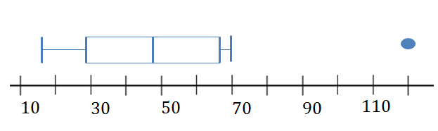
If a data value is very far away from the quartiles, instead of being shown using the whiskers of the box-and-whisker plot, outliers are shown as separately plotted points. The whiskers are then drawn to the minimum and maximum values that are not outliers.
Note
When you have access to the internet watch this video, which explains how to draw a box-and-whisker plot for a data set.
Example 2.2
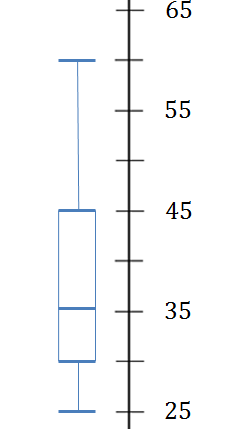
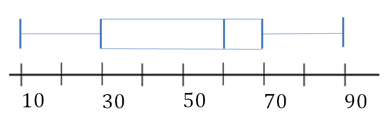
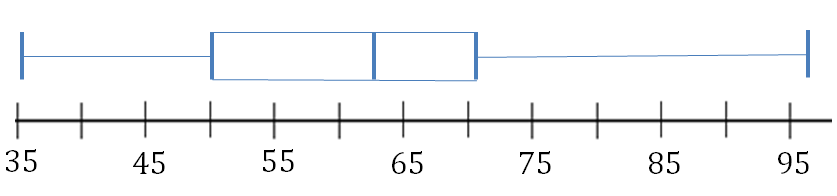
Determine the five-number summary and inter-quartile range from the box-and-whisker plot below.
Solution
We can read off the values for the five-number summary from the box plot.
[latex]\scriptsize \begin{align*}\text{Min}=25\\{{\text{Q}}_{1}}=30\\{{\text{Q}}_{2}}(\text{median})=35\\{{\text{Q}}_{3}}=45\\\text{Max}=60\end{align*}[/latex]
The upper quartile minus the lower quartile gives the inter-quartile range.
[latex]\scriptsize \begin{align*}\text{IQR}&=45-30\\&=15\end{align*}[/latex]
Exercise 2.1
- The stem-and-leaf diagram below shows the pulse rate per minute of ten learners.
[latex]\scriptsize \displaystyle 7[/latex] [latex]\scriptsize \displaystyle 8[/latex] [latex]\scriptsize \displaystyle 8[/latex] [latex]\scriptsize \displaystyle 1[/latex] [latex]\scriptsize \displaystyle 3[/latex] [latex]\scriptsize \displaystyle 5[/latex] [latex]\scriptsize \displaystyle 5[/latex] [latex]\scriptsize \displaystyle 9[/latex] [latex]\scriptsize \displaystyle 0[/latex] [latex]\scriptsize \displaystyle 1[/latex] [latex]\scriptsize \displaystyle 1[/latex] [latex]\scriptsize \displaystyle 10[/latex] [latex]\scriptsize \displaystyle 3[/latex] [latex]\scriptsize \displaystyle 5[/latex] - Determine the mean and the range of the data.
- Give the five-number summary and create a box plot for the data.
- The following is a list of data: [latex]\scriptsize \displaystyle 3;\text{ }8;\text{ }8;\text{ }5;\text{ }9;\text{ }1;\text{ }4;\text{ }x[/latex]
In each case, determine the value of [latex]\scriptsize x[/latex] if the:- range [latex]\scriptsize \displaystyle =16[/latex]
- mode [latex]\scriptsize =8[/latex]
- median[latex]\scriptsize =6[/latex]
- mean[latex]\scriptsize \displaystyle =6[/latex]
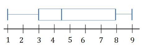
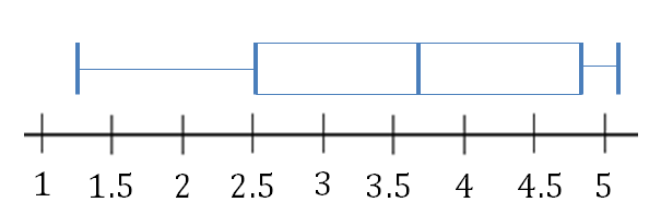
- box plot looks as follows:
- Given the following data set:
[latex]\scriptsize \displaystyle 1.25\text{ };\text{ }1.5\text{ };\text{ }2.5\text{ };\text{ }2.5\text{ };\text{ }3.1\text{ };\text{ }3.2\text{ };\text{ }4.1\text{ };\text{ }4.25\text{ };\text{ }4.75\text{ };\text{ }4.8\text{ };\text{ }4.95\text{ };\text{ }5.1[/latex]- Draw the box plot.
- Find the upper and lower fences of the data.
The full solutions are at the end of the unit.
Activity 2.2: Interpreting the box-and whisker plot
Time required: 20 minutes
What you need:
- a pen and paper
What to do:
In Activity 2.1 you saw that the marks of eight learners gave the following box plot:
- .
What percentage of learners scored below [latex]\scriptsize \displaystyle 66.5[/latex]? - How many learners scored below [latex]\scriptsize \displaystyle 66.5[/latex]?
- Between what two marks does the middle [latex]\scriptsize \displaystyle 50\%[/latex]of the data lie?
- What mark did [latex]\scriptsize \displaystyle 50\%[/latex] of learners score less than?
- Complete this sentence: Twenty-five percent of learners got a mark greater than________.
- What percentage of learners scored below [latex]\scriptsize \displaystyle 87.5[/latex]?
- Comment on the symmetry of the data values.
- Comment on the variability of the data.
What did you find?
- Twenty-five percent of scores fall below the lower quartile value.
- [latex]\scriptsize 0.25\times 8=2[/latex] So [latex]\scriptsize 2[/latex] learners got less than [latex]\scriptsize \displaystyle 66.5[/latex].
- The IQR shows the middle [latex]\scriptsize \displaystyle 50\%[/latex] of scores, therefore [latex]\scriptsize \displaystyle 50\%[/latex] of the data lies between [latex]\scriptsize \displaystyle 66.5[/latex] and [latex]\scriptsize \displaystyle 87.5[/latex].
- Half the scores are greater than or equal to the median and half are less than the median. [latex]\scriptsize \displaystyle 50\%[/latex] of learners got less than [latex]\scriptsize \displaystyle 76[/latex].
- Twenty-five percent of learners got a mark greater than [latex]\scriptsize 87.5[/latex].
- Seventy-five percent of learners scored less than [latex]\scriptsize \displaystyle 87.5[/latex].
- The data appears to be more or less symmetric as the median lies close to the middle of the box.
- Consider the range and IQR. The range is easily influenced by extreme values and outliers so it is less reliable than the IQR, which takes into account only the middle [latex]\scriptsize \displaystyle 50\%[/latex] of the data.
.
[latex]\scriptsize \begin{align*}\text{IQR}&=87.5-66.5\\&=21\\\text{Range}&=92-56\\&=36\end{align*}[/latex]
.
Low variability is ideal because it means that you can make better predictions about the population based on sample data. High variability means that the values are less consistent, so it’s more difficult to make predictions.
We can say that the marks are moderately variable.
When data are skewed, the majority of the data values are located either on the high or low ends. The shape of a box-and-whisker plot will show if a data set is normally distributed or skewed.
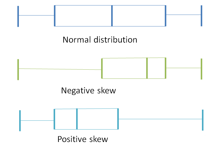
When the median is in the middle of the box, and the whiskers are about the same length on either side of the box, then the distribution is symmetric or normal.
When the median is pulled toward the upper quartile, and the whisker is shorter on the upper end of the box, then the distribution is negatively skewed (skewed left).
When the median is pulled toward the lower quartile, and the whisker is shorter on the lower end of the box, then the distribution is positively skewed (skewed right).
Note
For more on interpreting box plots watch this video called “Interpreting box plots”.
Summary
In this unit you have learnt the following:
- How to define the five-number summary.
- How to represent the five-number summary using a box-and-whisker plot.
- How to interpret a box plot.
- How the median is affected by negatively and positively skewed data.
Unit 2: Assessment
Suggested time to complete: 30 minutes
- Two mathematics classes, A and B, are in competition to see which class performed best in the June examination. The marks of the learners in class A are given below and the box-and-whisker plot for class B illustrates the results of class B. Both classes have 25 learners. Marks are given as percentages.
Marks of class A:
[latex]\scriptsize \displaystyle 9;\text{ }14;\text{ }14;\text{ }19;\text{ }21;\text{ }23;\text{ }33;\text{ }35;\text{ }37;\text{ }37;\text{ }42;\text{ }45;\text{ }55;\text{ }56;\text{ }57;\text{ }59;\text{ }68;\text{ }75;\text{ }75;\text{ }75;\text{ }77;\text{ }78;\text{ }80;\text{ }81;\text{ }92[/latex]
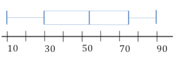
The box and whisker diagram for the learners in class B is:
- Write down the five-number summary for class A.
- Are there any outliers in the data for class A? Explain.
- Draw the box-and-whisker diagram (box plot) for class A. Show all relevant values.
- Determine which class did better in the June Examination and give reasons for your conclusion.
- The ages of 28 people whose birthday coincides with that of one of their children are shown below.
[latex]\scriptsize \displaystyle \begin{align*}&78;\text{ }53;\text{ }70;\text{ }97;\text{ }37;\text{ }68;\text{ }48;\text{ }35;\text{ }71;\text{ }63;\text{ }47;\text{ }60;\text{ }63;\text{ }58;\\&74;\text{ }39;\text{ }67;\text{ }64;\text{ }42;\text{ }52;\text{ }38;\text{ }54;\text{ }60;\text{ }75;\text{ }69;\text{ }77;\text{ }65;\text{ }72\end{align*}[/latex]- Determine the median age of the group by first determining its position.
- Determine the upper and lower quartiles of the data by first determining their positions.
- Determine the upper and lower fence values.
- Construct a box-and-whisker diagram for the above information showing any outliers.
- Test scores for a college statistics class held during the day are:
[latex]\scriptsize \displaystyle \begin{align*}99;\text{ }56;\text{ }78;\text{ }55.5;\text{ }32;\text{ }90;\text{ }80;\text{ }81;\text{ }56;\text{ }59;\text{ }45;\text{ }77;\text{ }84.5;\text{ }84;\text{ }70;\text{ }72;\text{ }68;\text{ }32;\text{ }79;\text{ }90\end{align*}[/latex]
Test scores for a college statistics class held during the evening are:
[latex]\scriptsize \displaystyle \begin{align*}98;\text{ }78;\text{ }68;\text{ }83;\text{ }81;\text{ }89;\text{ }88;\text{ }76;\text{ }65;\text{ }45;\text{ }98;\text{ }90;\text{ }80;\text{ }84.5;\text{ }85;\text{ }79;\text{ }78;\text{ }98;\text{ }90;\text{ }79;\text{ }81;\text{ }25.5\end{align*}[/latex]- For each data set, what percentage of the data is between:
- the smallest value and the first quartile?
- the first quartile and the median?
- the median and the third quartile?
- the third quartile and the largest value?
- the first quartile and the largest value?
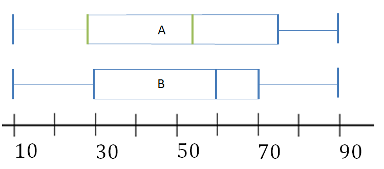
- Create a box plot for each set of data. Use one number line for both box plots.
- Which box plot has the widest spread for the middle [latex]\scriptsize \displaystyle 50\%[/latex] of the data? What does this mean for that set of data in comparison to the other set of data?
- For each data set, what percentage of the data is between:
The full solutions are at the end of the unit.
Unit 2: Solutions
Exercise 2.1
- .
- .
[latex]\scriptsize \begin{align*}\bar{x}&=\displaystyle \frac{{78+81+83+2(85)+90+(2)91+103+105}}{{10}}\\&=\displaystyle \frac{{892}}{{10}}\\&=89.2\end{align*}[/latex]
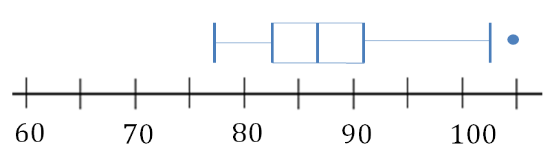
[latex]\scriptsize \begin{align*}\text{Range}&=105-78\\&=27\end{align*}[/latex] - Five number summary:
[latex]\scriptsize \begin{align*}\{78;\text{ }&81;\text{ }83;\text{ }85;\text{ }85;\text{ }90;\text{ }91;\text{ }91;\text{ }103;\text{ }105\}\\\text{Min}&=78\\{{\text{Q}}_{1}}&=83\\\text{Median}&=87.5\\{{\text{Q}}_{3}}&=91\\\text{Max}&=105\end{align*}[/latex]
.
There is an outlier in this data set:
[latex]\scriptsize \begin{align*}\text{IQR}&=91-83\\&=8\\\text{Upper fence}&={{\text{Q}}_{3}}+1.5(\text{IQR})\\&=91+1.5(8)\\&=103\end{align*}[/latex]
[latex]\scriptsize 105[/latex] is an outlier.
- .
- .
- .
[latex]\scriptsize \begin{align*}x-1&=16\\x&=17\end{align*}[/latex] - [latex]\scriptsize x\in \mathbb{Z},\text{ }x\ne 1;3;4;5;9[/latex]
[latex]\scriptsize x[/latex] can be any integer value that will not change the mode of [latex]\scriptsize 8[/latex] so we must exclude all other values in the data set. - The median will be between positions [latex]\scriptsize 4[/latex] and [latex]\scriptsize 5[/latex]
[latex]\scriptsize \begin{align*}\displaystyle \frac{{5+x}}{2}&=\text{M}\\x&=6\times 2-5\\&=7\end{align*}[/latex] - .
[latex]\scriptsize \displaystyle \begin{align*}\text{Mean}&=\displaystyle \frac{{1+3+4+5+8+8+9+x}}{8}\\&=6\\\displaystyle \frac{{x+38}}{8}&=6\\x&=10\end{align*}[/latex] - .
[latex]\scriptsize \begin{align*}\text{Median}&=4.5\\\displaystyle \frac{{x+5}}{2}&=4.5\\x&=4\end{align*}[/latex]
- .
- .
- .
[latex]\scriptsize \displaystyle \begin{align*}\text{Min}&=1.25\\{{\text{Q}}_{1}}&=2.5\\{{\text{Q}}_{2}}&=3.65\\{{\text{Q}}_{3}}&=4.78\\\text{Max}&=5.1\end{align*}[/latex]
- .
[latex]\scriptsize \begin{align*}\text{IQR}&=4.78-2.5\\&=2.28\\\text{Lower fence}&={{\text{Q}}_{1}}-1.5(2.28)\\&=2.5-1.5(2.28)\\&=-0.92\\\text{Upper fence}&={{\text{Q}}_{3}}+1.5(2.28)\\&=4.78+1.5(2.28)\\&=8.2\end{align*}[/latex]
- .
Unit 2: Assessment
- .
- [latex]\scriptsize \displaystyle \text{min}=9;\text{ first quartile}=28;\text{ median}=55;\text{ third quartile}=75;\text{ max}=92[/latex]
- All values fall within the lower and upper fences so there are no outliers.
- .
- Compare the box-and-whisker plots for the classes.
Class B did marginally better than class A. Its median is [latex]\scriptsize \displaystyle 60[/latex] while class A’s is [latex]\scriptsize \displaystyle 55[/latex]. Furthermore, the first quartile for class B is higher than that of class A.
- .
- First sort the data then calculate the position of the median age.
[latex]\scriptsize \displaystyle \begin{align*}&35;\text{ }37;\text{ }38;\text{ }39;\text{ }42;\text{ }47;\text{ }48;\text{ }52;\text{ }53;\text{ }54;\text{ }58;\text{ }60;\text{ }60;\text{ }63\\&63;\text{ }64;\text{ }65;\text{ }67;\text{ }68;\text{ }69;\text{ }70;\text{ }71;\text{ }72;\text{ }74;\text{ }75;\text{ }77;\text{ }78;\text{ }97\end{align*}[/latex]
The median will be between positions [latex]\scriptsize 14[/latex] and [latex]\scriptsize 15[/latex].
[latex]\scriptsize \text{Median age }=63[/latex] - The lower quartile lies between positions [latex]\scriptsize 7[/latex] and [latex]\scriptsize 8[/latex].
[latex]\scriptsize \begin{align*}{{\text{Q}}_{1}}&=\displaystyle \frac{{48+52}}{2}\\&=50\end{align*}[/latex]
.
The upper quartile lies between positions [latex]\scriptsize 21[/latex] and [latex]\scriptsize 22[/latex].
[latex]\scriptsize \begin{align*}{{\text{Q}}_{3}}&=\displaystyle \frac{{70+71}}{2}\\&=70.5\end{align*}[/latex] - .
[latex]\scriptsize \begin{align*}\text{IQR}&=70.5-50\\&=20.5\\\text{Upper fence}&={{\text{Q}}_{3}}+1.5(\text{IQR})\\&=70.5+1.5(20.5)\\&=101.25\\\text{Lower fence}&={{\text{Q}}_{1}}-1.5(\text{IQR})\\&=50-1.5(20.5)\\&=19.25\end{align*}[/latex] - .
There are no outliers.
- First sort the data then calculate the position of the median age.
- .
- Order the data for each group.
Day class:
[latex]\scriptsize \displaystyle 32;\text{ }32;\text{ }45;\text{ }55.5;\text{ }56;\text{ }56;\text{ }59;\text{ }68;\text{ }70;\text{ }72;\text{ }77;\text{ }78;\text{ }79;\text{ }80;\text{ }81;\text{ }84;\text{ }84.5;\text{ }90;\text{ }90;\text{ }99[/latex]
.
There are twenty data values for the day class and the five-number-summary is:
[latex]\scriptsize \displaystyle \begin{align*}\text{Min}&=32\\{{\text{Q}}_{\text{1}}}&=56\\{{\text{Q}}_{2}}&=74.5\\{{\text{Q}}_{\text{3}}}&=82.5\\\text{Max}&=99\end{align*}[/latex]- There are six data values ranging from the minimum to the first quartile so [latex]\scriptsize 30\%[/latex] of data values lie between [latex]\scriptsize 32[/latex] and [latex]\scriptsize 56[/latex].
- There are six data values ranging from [latex]\scriptsize 56[/latex] to [latex]\scriptsize 74.5[/latex] so [latex]\scriptsize 30\%[/latex] of the data values lie between the first quartile and the median.
- There are five data values ranging from [latex]\scriptsize 74.5[/latex] to [latex]\scriptsize 82.5[/latex] so [latex]\scriptsize 25\%[/latex] of data values lie between the median and the third quartile.
- There are five data values ranging from [latex]\scriptsize 82.5[/latex] to [latex]\scriptsize 99[/latex], which is [latex]\scriptsize 25\%[/latex] of the data.
- There are [latex]\scriptsize 15[/latex] data values between the first quartile, [latex]\scriptsize 56[/latex], and the largest value, [latex]\scriptsize 99[/latex], this is [latex]\scriptsize 75\%[/latex] of the data.
Night class:
[latex]\scriptsize \displaystyle 25.5;\text{ }45;\text{ }65;\text{ }68;\text{ }76;\text{ }78;\text{ }78;\text{ }79;\text{ }79;\text{ }80;\text{ }81;\text{ }81;\text{ }83;\text{ }84.5;\text{ }85;\text{ }88;\text{ }89;\text{ }90;\text{ }90;\text{ }98;\text{ }98;\text{ }98[/latex]
.
There are twenty-two data values for the evening class and the five-number-summary is:
[latex]\scriptsize \displaystyle \begin{align*}\text{Min}&=25.5\\{{\text{Q}}_{\text{1}}}&=78\\{{\text{Q}}_{2}}&=81\\{{\text{Q}}_{\text{3}}}&=89\\\text{Max}&=98\end{align*}[/latex]- There are six data values ranging from the minimum to the first quartile so approximately [latex]\scriptsize 27\%[/latex] of data values.
- There are five data values ranging from the first quartile to the median so approximately [latex]\scriptsize 23\%[/latex] of data values.
- There are six data values ranging from the median to the third quartile so approximately [latex]\scriptsize 27\%[/latex] of data values.
- There are five data values ranging from the third quartile to the maximum so approximately [latex]\scriptsize 23\%[/latex] of data values.
- There are sixteen data values ranging from the first quartile to the maximum so approximately [latex]\scriptsize 73\%[/latex] of data values.
- .
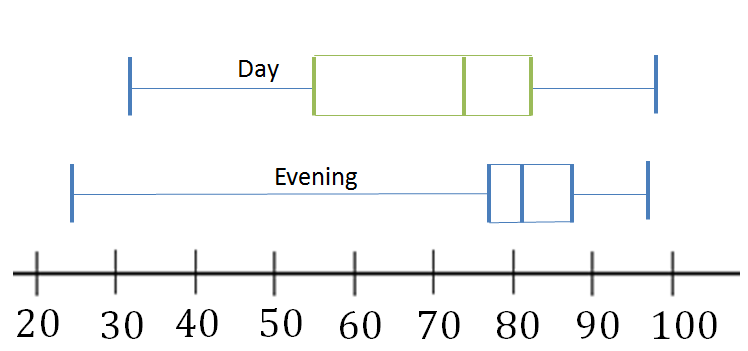
- The day class has the wider spread for the middle [latex]\scriptsize 50\%[/latex] of the data. The IQR for the day class data is greater than the IQR for the evening class. This means that there is more variability in the day class data.
- Order the data for each group.
Media Attributions
- Fig 1_Activity 2.1 Box and whisker © DHET is licensed under a CC BY (Attribution) license
- Fig 2_Key parts of box and whisker diagram © DHET is licensed under a CC BY (Attribution) license
- Fig 3_Example 2.1_Draw box and whisker © DHET is licensed under a CC BY (Attribution) license
- Fig 4_Example 2.2 Interpret Box and whisker © DHET is licensed under a CC BY (Attribution) license
- Fig 5_Ex 2.1 Q1eBox and whisker © DHET is licensed under a CC BY (Attribution) license
- Fig 8_Shape of box plots © DHET is licensed under a CC BY (Attribution) license
- Fig 9_Assessment Q1 © DHET is licensed under a CC BY (Attribution) license
- Fig 6_Exercise 2.1 Q1 Ans b © DHET is licensed under a CC BY (Attribution) license
- Fig 7_Ex 2.1 Q3Ans © DHET is licensed under a CC BY (Attribution) license
- Fig10_Assessment Q1c © DHET is licensed under a CC BY (Attribution) license
- Fig 11 Assessment Q1d © DHET is licensed under a CC BY (Attribution) license
- Fig 12_Assessment Ans 2d © DHET is licensed under a CC BY (Attribution) license
- Fig 13_Assessment Ans 3b © DHET is licensed under a CC BY (Attribution) license
