Financial mathematics: Use simple and compound interest to explain and define a variety of situations
Unit 3: Using timelines for calculations of simple and compound interest
Unit outcomes
By the end of this unit you will be able to:
- Interpret financial questions using timelines.
What you should know
Before you start this unit, make sure that you can:
- Use a scientific calculator. Look back to level 2 subject outcome 1.1 to revise this.
- Make calculations involving simple interest.
- Make calculations using compound interest.
For help with calculations of simple and compound interest, and the distinctions between these, you could review:
Introduction
In units 1 and 2 of this subject outcome, you have seen how to calculate with the simple and compound interest formulae. You have also done calculations to investigate variations on the compound growth formula that involve different rates of compounding.
Very often, changes are made to investments and loans during the course of the period of the investment or loan, and these have the effect of changing the details of the formulae that should be used for parts of that investment period.
For example, an investor may need to withdraw a portion of their investment for an emergency expense, or may have an unexpected windfall, which may allow them to invest an additional amount for part of the period.
A timeline is useful for representing this information when there are changes to the variables ([latex]\scriptsize A\text{, }P[/latex] and [latex]\scriptsize i[/latex] ) during the period of the investment or the loan.
Using time lines to illustrate changes made to investments or loans over their period
You will need to use the statement of each given problem to draw a line that represents the entire duration of the investment from the first deposit/loan to the end, whether it ends with a withdrawal or a final repayment. The line is marked off, usually in periods of years, although this depends on the calculations to be made. Interest rates, and amounts of deposits or loans, and changes in these, are indicated against the line. Let’s take a look at an example.
Example 3.1
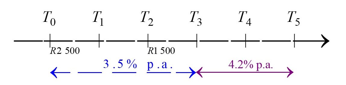
[latex]\scriptsize \text{R}2\text{ 500}[/latex] is invested for two years in a savings account at [latex]\scriptsize 3.5\text{ }\% \text{ }[/latex] compound interest per annum. After that period, a further [latex]\scriptsize \text{R}1\text{ }500[/latex] is deposited into the account. The interest rate is adjusted to [latex]\scriptsize 4.2\text{ }\%[/latex] compound interest per annum at the end of the third year. Calculate the total amount in the account after a total period of five years, if no further adjustments are made.
Solution
The timeline drawn below shows the initial deposit of [latex]\scriptsize \text{R}2\text{ }500[/latex] at [latex]\scriptsize {{T}_{0}}[/latex] (the start of the investment period), with the entire investment period from [latex]\scriptsize {{T}_{0}}[/latex] to [latex]\scriptsize {{T}_{5}}[/latex] – the five-year period. After two years, represented by [latex]\scriptsize {{T}_{2}}[/latex], the deposit of [latex]\scriptsize \text{R}1\text{ }500[/latex] is shown: all deposits are aligned in the timeline diagram.
Interest rates are shown with arrows extending over the period for which they are relevant: so the rate of [latex]\scriptsize 3.5\text{ }\% \text{ }[/latex] compound interest per annum is paid from the start to the end of the third year – from [latex]\scriptsize {{T}_{0}}[/latex] to [latex]\scriptsize {{T}_{3}}[/latex], when it changes to [latex]\scriptsize 4.2\text{ }\%[/latex] compound interest per annum for the remainder of the investment period.
In the calculations, investments are treated separately.
Period 1:
In the period [latex]\scriptsize {{T}_{0}}[/latex] to [latex]\scriptsize {{T}_{2}}[/latex], the investment consists of [latex]\scriptsize \text{R}2\text{ 500}[/latex] invested at [latex]\scriptsize 3.5\text{ }\% \text{ }[/latex] p.a. compound interest per annum.
[latex]\scriptsize \begin{align*}{{A}_{1}}&={{P}_{1}}{{\left( {1+i} \right)}^{n}}\\&=2\text{ }500{{\left( {1+0.035} \right)}^{2}}\\&=2\text{ }500\left( {1.071225} \right)\\&=2\text{ }678.0625\end{align*}[/latex]
The investment had a value of [latex]\scriptsize \text{R}2\text{ }678.06[/latex] (correct to two decimal places) at the end of the second year. To avoid introducing round-off errors, we prefer to use [latex]\scriptsize {{A}_{1}}=2\text{ }500{{(1+0.035)}^{2}}[/latex] in subsequent calculations.
Period 2:
In the period [latex]\scriptsize {{T}_{2}}[/latex] to [latex]\scriptsize {{T}_{3}}[/latex], there was a further deposit of [latex]\scriptsize \text{R}1\text{ 500}[/latex]. While the interest rate remained the same for one more year, substituting the expression for [latex]\scriptsize {{A}_{1}}[/latex] shows that the principal after [latex]\scriptsize {{T}_{2}}[/latex], at the start of the third year was
[latex]\scriptsize \begin{align*}{{P}_{2}}&=1\text{ }500+{{A}_{1}}\\&=1\text{ }500+2\text{ }500{{(1+0.035)}^{2}}\end{align*}[/latex]
Using this in the compound interest formula for this second period, we arrive at an expression of the value of the investment by the end of the third year:
[latex]\scriptsize \begin{align*}{{A}_{2}}&={{P}_{2}}{{\left( {1+i} \right)}^{n}}\\&=\left[ {1\text{ }500+2\text{ }500{{{\left( {1+0.035} \right)}}^{2}}} \right]{{\left( {1+0.035} \right)}^{1}}\\&=\left[ {4\text{ }178.0625} \right](1.035)\\&=4\text{ }324.294688\end{align*}[/latex]
The investment had a value of [latex]\scriptsize \text{R4 324}.30[/latex] (correct to two decimal places) at the end of the third year. So [latex]\scriptsize {{P}_{3}}={{A}_{2}}[/latex].
Once again, to avoid introducing round-off errors, we prefer to use [latex]\scriptsize {{A}_{2}}=\left[ {1\text{ }500+2\text{ }500{{{(1+0.035)}}^{2}}} \right]{{(1+0.035)}^{1}}[/latex] in subsequent calculations.
Period 3:
In the remaining two years from [latex]\scriptsize {{T}_{3}}[/latex] to [latex]\scriptsize {{T}_{5}}[/latex], the interest rate was increased to [latex]\scriptsize 4.2\text{ }\% \text{ }[/latex] compound interest per annum. The value of the investment after the period of five years will be:
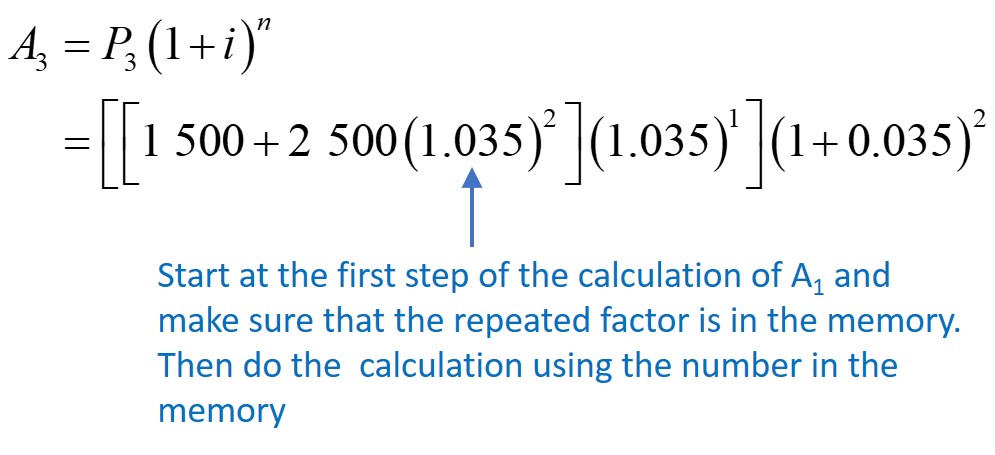
[latex]\scriptsize \begin{align*}{{A}_{3}}&={{P}_{3}}{{\left( {1+i} \right)}^{n}}\\&=\left[ {\left[ {1\text{ }500+2\text{ }500{{{\left( {1.035} \right)}}^{2}}} \right]{{{\left( {1.035} \right)}}^{1}}} \right]{{\left( {1+0.035} \right)}^{2}}\\&=\left[ {\left[ {4\text{ }178.0625} \right]{{{\left( {1.035} \right)}}^{1}}} \right]{{\left( {1.042} \right)}^{2}}\\&=\left[ {4\text{ }324.294688} \right]{{(1.042)}^{2}}\\&=4\text{ }695.163497\\&=\text{R}4\text{ 695}.16\end{align*}[/latex]
The value of the investment at the end of the five year period is [latex]\scriptsize \text{R}4\text{ }695.16[/latex].
You will see from the example above that it is only necessary to work out the answer to the calculation in the final step.
Take note!
It’s important to know how to use your calculator memory in complicated calculations.
(These instructions are for a CASIO fx-991ES PLUS calculator. They might also work for your later model CASIO, or SHARP calculators. If not, you need to refer to an operating manual for your calculator.)
Although each subsection of the calculation can be worked out completely, it is inconvenient, and sometimes impossible, to write down long, trailing decimal fractions. Rounding answers off for each part of the calculation might lead to round-off errors in your final answer. It is best to build up the calculation using the timeline, until you have all its parts, and then to work out the answer, rounding off only the final number.
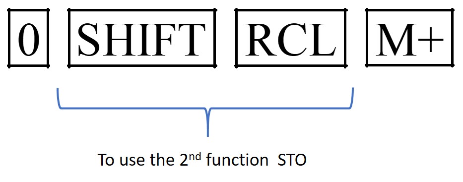
Your calculator’s memory function can be very useful in long calculations that use a repeated factor. For example, in the above calculation of [latex]\scriptsize {{A}_{3}}[/latex] it is useful to store the [latex]\scriptsize 1+i=1.035[/latex] in the memory. Key the following into your calculator to do so (making sure that the value in the calculator memory is 0 before you start):
![]()
This stores [latex]\scriptsize 1.035[/latex] in the memory, and clears the screen for your calculation.
To recall what is stored in the memory, press the following keys:
![]()
This brings the value in the memory to the screen, ready to be used immediately in the calculation. So, once you have worked out what to calculate for [latex]\scriptsize {{A}_{3}}[/latex], you could proceed as follows:

After you have written down your answer, you need to clear your calculator screen AND memory for the next calculation. This is how to clear the calculator memory:
Example 3.2
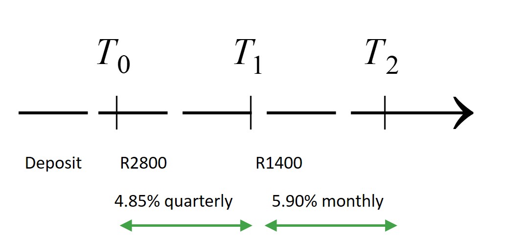
[latex]\scriptsize \text{R}2\text{ }8\text{00}[/latex] is invested in a savings account and [latex]\scriptsize 12[/latex] months later, a further [latex]\scriptsize \text{R}1\text{ }400[/latex] is deposited into the account. Calculate the total amount saved by the end of the second year if the interest rate is [latex]\scriptsize 4.85\text{ }\% \text{ }[/latex]compounded quarterly for the first year, and is then adjusted to [latex]\scriptsize 5.90\text{ }\% \text{ }[/latex] compounded monthly for the second year.
Solution
The timeline below shows the deposits and interest rates over the entire [latex]\scriptsize {{T}_{0}}\text{ to }{{T}_{2}}[/latex] two-year period.
Period 1:
Consider the first deposit:
[latex]\scriptsize \begin{align*}{{A}_{1}}&=P{{\left( {1+\displaystyle \frac{r}{{100\times m}}} \right)}^{{t\times m}}}\\&=2\text{ }800{{\left( {1+\displaystyle \frac{{4.85}}{{100\times 4}}} \right)}^{{1\times 4}}}\end{align*}[/latex]
This is the expression for the total value of the first investment after one year.
Period 2:
The second deposit is added to this amount at [latex]\scriptsize {{T}_{1}}[/latex], and the interest rate is changed.
[latex]\scriptsize {{P}_{2}}=1\text{ }400+{{A}_{1}}[/latex]
[latex]\scriptsize \begin{align*}{{A}_{2}}&={{P}_{2}}{{\left( {1+\displaystyle \frac{r}{{100\times m}}} \right)}^{{t\times m}}}\\&=\left[ {1\text{ }400+2\text{ }800{{{\left( {1+\displaystyle \frac{{4.85}}{{400}}} \right)}}^{4}}} \right]{{\left( {1+\displaystyle \frac{{5.90}}{{100\times 12}}} \right)}^{{1\times 12}}}\\&=\left[ {1\text{ }400+2\text{ }800{{{\left( {1.012125} \right)}}^{4}}} \right]{{\left( {1+\displaystyle \frac{{5.90}}{{100\times 12}}} \right)}^{{1\times 12}}}\\&=4\text{ }338.29{{\left( {1+0.00491667} \right)}^{{12}}}\\&=4\text{ }338.29{{\left( {1.00491667} \right)}^{{12}}}\\&=\text{R}4\text{ }601.29\end{align*}[/latex]
Exercise 3.1
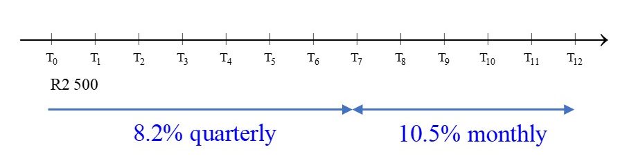
- [latex]\scriptsize \text{R}2\text{ }500[/latex] is deposited in a savings account for [latex]\scriptsize 12[/latex] years. For the first seven years, the interest rate is [latex]\scriptsize 8.2\text{ }\% \text{ }[/latex] p.a. compounded quarterly, and then it is increased to [latex]\scriptsize 10.5\text{ }\% \text{ }[/latex] p.a. compounded monthly.
- Use a timeline to show the status of the investment.
- Calculate the amount of money accumulated by the end of [latex]\scriptsize 12[/latex] years.
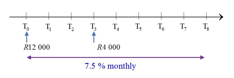
- [latex]\scriptsize \text{R}12\text{ 000}[/latex] is deposited into a savings account, and three years later, a further deposit of [latex]\scriptsize \text{R}4\text{ 000}[/latex] is added to the savings. Calculate the amount of money in the savings account at the end of eight years if the interest rate is [latex]\scriptsize 7.5\text{ }\%[/latex] compounded monthly.
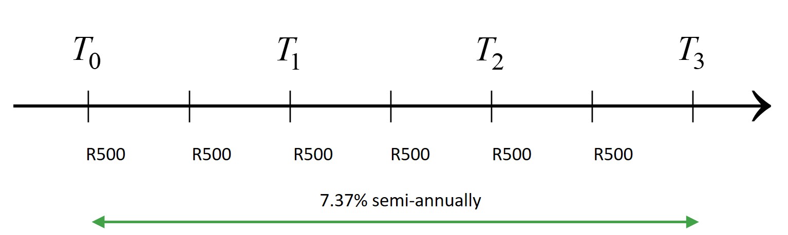
- Every six months for three years [latex]\scriptsize \text{R}500[/latex] is deposited into a Fixed Deposit savings account, with the first deposit made immediately, and the sixth and final deposit made six months before the end of the third year. Calculate the value of the investment at the end of the third year, assuming a [latex]\scriptsize 7.37\text{ }\% \text{ }[/latex] interest rate, compounded semi-annually.
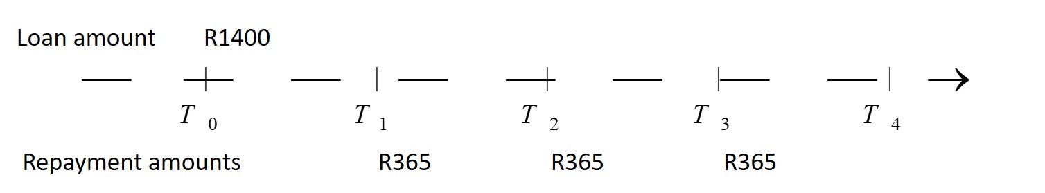
- Nonhlanhla borrowed [latex]\scriptsize \text{R}1\text{ }400[/latex], and repaid [latex]\scriptsize \text{R}365[/latex] at the end of the first year, and made two further instalments of [latex]\scriptsize \text{R}365[/latex] at the end of the second and third years. If a simple interest rate of [latex]\scriptsize 11\text{ }\% \text{ }[/latex] is charged on the loan, use a timeline to show how you calculate what amount must be repaid to settle the debt at the end of the fourth year.
- [latex]\scriptsize \displaystyle \text{R}50\text{ 000}[/latex] is deposited into a savings account, and [latex]\scriptsize 18[/latex] months later [latex]\scriptsize \text{R}12\text{ 000}[/latex] is withdrawn from the account. How much money will be in the account at the end of five years if the interest is calculated at [latex]\scriptsize 8[/latex]% compounded quarterly?
- [latex]\scriptsize \text{R}75\text{ 000}[/latex] is invested in the bond market for nine years. The interest rate for the first three years is [latex]\scriptsize 8.5\text{ }\%[/latex] compounded annually. For the next four years the interest rate increased to [latex]\scriptsize 9.75\text{ }\%[/latex] compounded quarterly. During the final two years, the interest rate is [latex]\scriptsize 10.25\text{ }\%[/latex] compounded monthly. Calculate the total value of the investment at the end of the nine years.
The full solutions are at the end of the unit.
Note
If you would like more worked examples, you can find some at this link.
Summary
In this unit you have learnt the following:
- How to interpret financial questions using timelines.
- How to use your calculator’s memory to do calculations using repeated factors.
Unit 3: Assessment
Suggested time to complete: 20 minutes
- [latex]\scriptsize \text{R}3\text{ 500}[/latex] is deposited into a savings account, and [latex]\scriptsize 18[/latex] months later [latex]\scriptsize \text{R}1\text{ 800}[/latex] is added to the amount. Calculate the total amount saved by the end of four years if the interest rate is [latex]\scriptsize 7.2\text{ }\%[/latex] compounded quarterly for the first year, and is then increased to [latex]\scriptsize 8.5\text{ }\%[/latex] compounded monthly for the remainder of the period. Use a timeline to show the changes to the investment over the time period.
- [latex]\scriptsize \text{R}10\text{ 200}[/latex] is deposited into a savings account, and two years later [latex]\scriptsize \text{R}4\text{ 500}[/latex] is withdrawn from the account. How much money will be in the account at the end of five years if the interest rate is [latex]\scriptsize 12.2\text{ }\%[/latex] compounded quarterly? Use a timeline to show the changes to the investment over the time period.
The full solutions are at the end of the unit.
Unit 3: Solutions
Exercise 3.1
- .
- The timeline for the investment can be drawn as follows:
- Consider the first deposit of [latex]\scriptsize \text{R}2\text{ }500[/latex].
At the end of seven years, the amount accumulated will be:
[latex]\scriptsize \begin{align*}{{A}_{1}}&={{P}_{1}}{{\left( {1+\displaystyle \frac{r}{{100\times m}}} \right)}^{{t\times m}}}\\&=2\text{ }500{{\left( {1+\displaystyle \frac{{8.2}}{{100\times 4}}} \right)}^{{7\times 4}}}\end{align*}[/latex]
.
Consider the second period of the saving account.
After seven years, the interest rate changes, so for the next five years, the interest rate is [latex]\scriptsize 10.5\text{ }\% \text{ }[/latex] p.a. compounded monthly.
.
At the start of this second period, the initial investment amount is the accumulated total from the first period. So, we could say that [latex]\scriptsize {{P}_{2}}={{A}_{1}}[/latex].
So, the total amount by the end of the [latex]\scriptsize 12[/latex] years will be:
[latex]\scriptsize \begin{align*}{{A}_{{Total}}}&={{P}_{2}}{{\left( {1+\displaystyle \frac{r}{{100\times m}}} \right)}^{{t\times m}}}\\&=\left[ {2\text{ }500{{{\left( {1+\displaystyle \frac{{8.2}}{{100\times 4}}} \right)}}^{{7\times 4}}}} \right]{{\left( {1+\displaystyle \frac{{10.5}}{{100\times 12}}} \right)}^{{5\times 12}}}\\&=\left[ {2\text{ }500{{{\left( {1.0205} \right)}}^{{28}}}} \right]{{\left( {1.00875} \right)}^{{60}}}\\&=\left( {4\text{ }412.699} \right)\left( {1.687} \right)\\&=\text{R}7\text{ 442}\text{.47}\end{align*}[/latex]
.
Comment: Notice that after [latex]\scriptsize 12[/latex] years of schooling, a child is eligible for tertiary education. Young parents are likely to start thinking about ways to save to pay for their children’s education when they start school. Although this investment would be a good contribution, it would not be enough to pay for tertiary education. Parents would do better to start saving when their children are younger (if possible) and to continue to save while they are at primary and secondary school.
- The timeline for the investment can be drawn as follows:
- .
Consider the first period:
[latex]\scriptsize \begin{align*}{{A}_{1}}&={{P}_{1}}{{\left( {1+\displaystyle \frac{r}{{100\times m}}} \right)}^{{t\times m}}}\\&=12\text{ }000{{\left( {1+\displaystyle \frac{{7.5}}{{100\times 12}}} \right)}^{{3\times 12}}}\\&=12\text{ }000{{\left( {1.00625} \right)}^{{36}}}\end{align*}[/latex]
.
Consider the second period:
The investment principal for this period is the amount accumulated by the end of the first period: [latex]\scriptsize {{P}_{2}}={{A}_{1}}[/latex]
[latex]\scriptsize \begin{align*}{{A}_{2}}&={{P}_{2}}{{\left( {1+\displaystyle \frac{r}{{100\times m}}} \right)}^{{t\times m}}}\\&=\left[ {12\text{ }000{{{\left( {1.00625} \right)}}^{{36}}}} \right]{{\left( {1.00625} \right)}^{{5\times 12}}}\\&=\left[ {15\text{ }017.35363} \right]{{\left( {1.00625} \right)}^{{60}}}\\&=21\text{ }824.63605\end{align*}[/latex]
At the end of eight years, there will be [latex]\scriptsize \text{R}21\text{ 824}\text{.64}[/latex] in the account. - .
There are different ways of approaching this problem:
Each deposit can be treated separately, and the individual amounts added together for the total value for the entire period.
1st deposit:
[latex]\scriptsize \begin{align*}A&=P{{\left( {1+\displaystyle \frac{r}{{100\times m}}} \right)}^{{t\times m}}}\\&=500{{\left( {1+\displaystyle \frac{{7.37}}{{100\times 2}}} \right)}^{{3\times 2}}}\\&=500{{\left( {1+0.03685} \right)}^{6}}\\&=\text{R}621.249\text{ correct to 3 decimal places}\end{align*}[/latex]
2nd deposit: Notice that the investment period for the second amount is 2.5 years.
[latex]\scriptsize \begin{align*}A&=P{{\left( {1+\displaystyle \frac{r}{{100\times m}}} \right)}^{{t\times m}}}\\&=500{{\left( {1+\displaystyle \frac{{7.37}}{{100\times 2}}} \right)}^{{2.5\times 2}}}\\&=500{{\left( {1+0.03685} \right)}^{5}}\\&=\text{R}599.169\text{ correct to 3 decimal places}\end{align*}[/latex]
3rd deposit:
[latex]\scriptsize \begin{align*}A&=P{{\left( {1+\displaystyle \frac{r}{{100\times m}}} \right)}^{{t\times m}}}\\&=500{{\left( {1+\displaystyle \frac{{7.37}}{{100\times 2}}} \right)}^{{2\times 2}}}\\&=500{{\left( {1+0.03685} \right)}^{4}}\\&=\text{R}577.875\text{ correct to 3 decimal places}\end{align*}[/latex]
4th deposit:
[latex]\scriptsize \begin{align*}A&=500{{\left( {1+\displaystyle \frac{{7.37}}{{100\times 2}}} \right)}^{{1.5\times 2}}}\\&=500{{\left( {1+0.03685} \right)}^{3}}\\&=\text{R}557.337\text{ correct to 3 decimal places}\end{align*}[/latex]
5th deposit:
[latex]\scriptsize \begin{align*}A&=500{{\left( {1+\displaystyle \frac{{7.37}}{{100\times 2}}} \right)}^{{1\times 2}}}\\&=500{{\left( {1+0.03685} \right)}^{2}}\\&=\text{R}537.529\text{ correct to 3 decimal places}\end{align*}[/latex]
6th deposit:
[latex]\scriptsize \begin{align*}A&=500{{\left( {1+\displaystyle \frac{{7.37}}{{100\times 2}}} \right)}^{{0.5\times 2}}}\\&=500{{\left( {1+0.03685} \right)}^{1}}\\&=\text{R}518.425\end{align*}[/latex]
The value of investment after three years is the sum of the values for all the deposits, which is [latex]\scriptsize \text{R}3\text{ }411.58[/latex]
.
Alternatively
1st deposit:
[latex]\scriptsize \begin{align*}{{A}_{1}}&={{P}_{1}}{{\left( {1+\displaystyle \frac{r}{{100\times m}}} \right)}^{{0.5\times m}}}\\&=500{{\left( {1+\displaystyle \frac{{7.37}}{{100\times 2}}} \right)}^{{0.5\times 2}}}\end{align*}[/latex]
2nd deposit:
At the start of the second period, the initial investment amount is the accumulated total from the first period with an additional [latex]\scriptsize R500[/latex]. So, we could say that [latex]\scriptsize {{P}_{2}}=500+{{A}_{1}}[/latex]. This second investment is also for a six-month period. So:
[latex]\scriptsize \begin{align*}{{A}_{2}}&={{P}_{2}}{{\left( {1+\displaystyle \frac{r}{{100\times m}}} \right)}^{{0.5\times m}}}\\&=\left[ {500+500{{{\left( {1+\displaystyle \frac{{7.37}}{{100\times 2}}} \right)}}^{{0.5\times 2}}}} \right]{{\left( {1+\displaystyle \frac{{7.37}}{{100\times 2}}} \right)}^{{0.5\times 2}}}\end{align*}[/latex]
3rd deposit:
At the start of the third period, the initial investment amount is the accumulated total from the second period with an additional [latex]\scriptsize \text{R}500[/latex]. So, we could say that [latex]\scriptsize {{P}_{3}}=500+{{A}_{2}}[/latex]. This third investment is also for a six-month period.
[latex]\scriptsize \begin{align*}{{A}_{3}}&={{P}_{3}}{{\left( {1+\displaystyle \frac{r}{{100\times m}}} \right)}^{{0.5\times m}}}\\&=\left[ {500+\left[ {500+500{{{\left( {1+\displaystyle \frac{{7.37}}{{100\times 2}}} \right)}}^{{0.5\times 2}}}} \right]{{{\left( {1+\displaystyle \frac{{7.37}}{{100\times 2}}} \right)}}^{{0.5\times 2}}}} \right]{{\left( {1+\displaystyle \frac{{7.37}}{{100\times 2}}} \right)}^{{0.5\times 2}}}\end{align*}[/latex]
And so on, as follows:
[latex]\scriptsize \begin{align*}{{A}_{4}}&={{P}_{4}}{{\left( {1+\displaystyle \frac{r}{{100\times m}}} \right)}^{{0.5\times m}}}\\&=\left[ {500+\left[ {500+\left[ {500+500{{{\left( {1+\displaystyle \frac{{7.37}}{{100\times 2}}} \right)}}^{{0.5\times 2}}}} \right]{{{\left( {1+\displaystyle \frac{{7.37}}{{100\times 2}}} \right)}}^{{0.5\times 2}}}} \right]{{{\left( {1+\displaystyle \frac{{7.37}}{{100\times 2}}} \right)}}^{{0.5\times 2}}}} \right]{{\left( {1+\displaystyle \frac{{7.37}}{{100\times 2}}} \right)}^{{0.5\times 2}}}\\\\{{A}_{5}}&=\left[ {500+\left[ {500+\left[ {500+\left[ {500+500{{{\left( {1+\displaystyle \frac{{7.37}}{{100\times 2}}} \right)}}^{{0.5\times 2}}}} \right]{{{\left( {1+\displaystyle \frac{{7.37}}{{100\times 2}}} \right)}}^{{0.5\times 2}}}} \right]{{{\left( {1+\displaystyle \frac{{7.37}}{{100\times 2}}} \right)}}^{{0.5\times 2}}}} \right]{{{\left( {1+\displaystyle \frac{{7.37}}{{100\times 2}}} \right)}}^{{0.5\times 2}}}} \right]{{\left( {1+\displaystyle \frac{{7.37}}{{100\times 2}}} \right)}^{{0.5\times 2}}}\end{align*}[/latex]
The formula for [latex]\scriptsize {{A}_{6}}[/latex] is getting far too long, so instead we can calculate the exact decimal value of the factor that increases the principal for each period: [latex]\scriptsize \begin{align*}{{A}_{6}}&=\left[ {500+\left[ {500+\left[ {500+\left[ {500+\left[ {500+500\left( {1.03685} \right)} \right]\left( {1.03685} \right)} \right]\left( {1.03685} \right)} \right]\left( {1.03685} \right)} \right]\left( {1.03685} \right)} \right]\left( {1.03685} \right)\\&=\left[ {500+\left[ {500+\left[ {500+\left[ {500+\left[ {500+518.425} \right]\left( {1.03685} \right)} \right]\left( {1.03685} \right)} \right]\left( {1.03685} \right)} \right]\left( {1.03685} \right)} \right]\left( {1.03685} \right)\\&=\left[ {500+\left[ {500+\left[ {500+\left[ {500+1\text{ }018.425\left( {1.03685} \right)} \right]\left( {1.03685} \right)} \right]\left( {1.03685} \right)} \right]\left( {1.03685} \right)} \right]\left( {1.03685} \right)\\&=\left[ {500+\left[ {500+\left[ {500+\left[ {500+1\text{ }055.953961} \right]\left( {1.03685} \right)} \right]\left( {1.03685} \right)} \right]\left( {1.03685} \right)} \right]\left( {1.03685} \right)\\&=\left[ {500+\left[ {500+\left[ {500+1\text{ }555.953961\left( {1.03685} \right)} \right]\left( {1.03685} \right)} \right]\left( {1.03685} \right)} \right]\left( {1.03685} \right)\\&=\left[ {500+\left[ {500+\left[ {500+1\text{ }613.290865} \right]\left( {1.03685} \right)} \right]\left( {1.03685} \right)} \right]\left( {1.03685} \right)\\&=\left[ {500+\left[ {500+2\text{ }113.2908525\left( {1.03685} \right)} \right]\left( {1.03685} \right)} \right]\left( {1.03685} \right)\\&=\left[ {500+\left[ {500+2\text{ }191.165633} \right]\left( {1.03685} \right)} \right]\left( {1.03685} \right)\\&=\left[ {500+2\text{ }691.165633\left( {1.03685} \right)} \right]\left( {1.03685} \right)\\&=\left[ {500+2\text{ }790.335087} \right]\left( {1.03685} \right)\\&=3\text{ }290.335087\left( {1.03685} \right)\\&=3\text{ }411.583935\\&=\text{R}3\text{ 411}\text{.58}\end{align*}[/latex]
.
This is obviously a case for using the calculator memory, which will simplify the workings. However, the first approach to the problem is more straightforward, with fewer opportunities for mistakes or confusion. - .
 .
.
Initial loan = [latex]\scriptsize \text{R}1\text{ }400[/latex]
Total amount owing at the end of the four years:
[latex]\scriptsize \begin{align*}&=P\left( {1+0.11\times 4} \right)\\&=1\text{ }400(1.44)\\&=\text{R}2\text{ }016\end{align*}[/latex]
.
The first repayment reduces the total loan by the amount repaid as well as the interest on that repayment amount for the remaining period of three years:
Reduction effect of 1st repayment: [latex]\scriptsize 365(1+0.11\times 3)=365(1.33)=\text{R}485.45[/latex]
.
Similarly, with subsequent repayments:
Reduction effect of 2nd repayment: [latex]\scriptsize 365\left( {1+0.11\times 2} \right)=365\left( {1.22} \right)=\text{R}445.30[/latex]
Reduction effect of 3rd repayment: [latex]\scriptsize 365\left( {1+0.11} \right)=365\left( {1.11} \right)=\text{R}405.15[/latex]
.
The outstanding amount to be settled at the end of the 4th year: [latex]\scriptsize 2\text{ }016-485.45-445.30-405.15=\text{R}680.10[/latex] - .
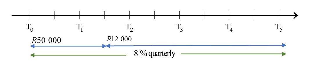
Consider the first period:
[latex]\scriptsize \begin{align*}{{A}_{1}}&={{P}_{1}}{{\left( {1+\displaystyle \frac{r}{{100\times m}}} \right)}^{{t\times m}}}\\&=50\text{ }000{{\left( {1+\displaystyle \frac{8}{{100\times 4}}} \right)}^{{1.5\times 4}}}\\&=50\text{ }000{{\left( {1.02} \right)}^{6}}\end{align*}[/latex]
.
Consider the second period:
At the start of the period, the principal will be the amount accumulated by the end of the first period: [latex]\scriptsize {{P}_{2}}={{A}_{1}}[/latex].
[latex]\scriptsize \begin{align*}{{A}_{2}}&={{P}_{2}}{{\left( {1+\displaystyle \frac{r}{{100\times m}}} \right)}^{{t\times m}}}\\&=\left[ {50\text{ }000{{{\left( {1.02} \right)}}^{6}}-12000} \right]{{\left( {1.02} \right)}^{{3.5\times 4}}}\\&=\left[ {44\text{ }308.12098} \right]{{\left( {1.02} \right)}^{{14}}}\\&=58\text{ }463.62\end{align*}[/latex]
.
By the end of five years, there will be [latex]\scriptsize \text{R}58\text{ 463}\text{.62}[/latex] in the account. - .
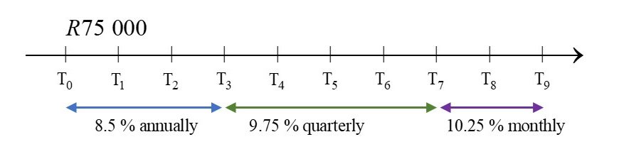
Consider the first period:
[latex]\scriptsize \begin{align*}{{A}_{1}}&={{P}_{1}}{{\left( {1+\displaystyle \frac{{8.5}}{{100\times 1}}} \right)}^{{3\times 1}}}\\&=75\text{ }000{{\left( {1.085} \right)}^{3}}\end{align*}[/latex]
.
Consider the second period:
The principal at the start of the second period is the accumulated amount of the first period: [latex]\scriptsize {{P}_{2}}={{A}_{1}}[/latex]
[latex]\scriptsize \begin{align*}{{A}_{2}}&={{P}_{2}}{{\left( {1+\displaystyle \frac{{9.75}}{{100\times 4}}} \right)}^{{4\times 4}}}\\&=\left[ {75\text{ }000{{{\left( {1.085} \right)}}^{3}}} \right]{{\left( {1.024375} \right)}^{{16}}}\end{align*}[/latex]
.
Consider the third period:
At the start of the third period, the principal will be the amount accumulated by the end of the second period: [latex]\scriptsize {{P}_{3}}={{A}_{2}}[/latex]
[latex]\scriptsize \begin{align*}{{A}_{3}}&={{P}_{3}}{{\left( {1+\displaystyle \frac{{10.25}}{{100\times 12}}} \right)}^{{2\times 12}}}\\&=\left[ {\left[ {75\text{ }000{{{\left( {1.085} \right)}}^{3}}} \right]{{{\left( {1.024375} \right)}}^{{16}}}} \right]{{\left( {1.008541...} \right)}^{{24}}}\\&=\left[ {\left[ {95\text{ }796.68...} \right]{{{\left( {1.024375} \right)}}^{{16}}}} \right]{{\left( {1.008541...} \right)}^{{24}}}\\&=\left[ {140\text{ }829.6217} \right]{{\left( {1.008541...} \right)}^{{24}}}\\&=172\text{ }721.4594\end{align*}[/latex]
At the end of the nine years, the total value of the investment will be [latex]\scriptsize \text{R}172\text{ 721}\text{.46}[/latex].
Unit 3: Assessment
- .
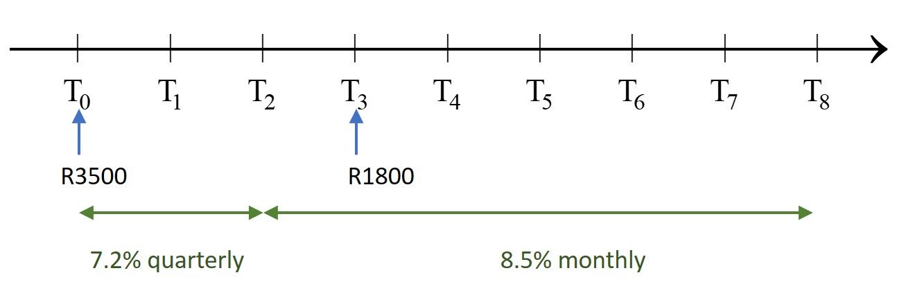 Consider the first period – the first year:
[latex]\scriptsize \begin{align*}{{A}_{1}}&={{P}_{1}}{{\left( {1+\displaystyle \frac{r}{{100\times m}}} \right)}^{{t\times m}}}\\&=3\text{ }500{{\left( {1+\displaystyle \frac{{7.2}}{{100\times 4}}} \right)}^{{1\times 4}}}\\&=3\text{ }500{{\left( {1.018} \right)}^{4}}\end{align*}[/latex]
.
Consider the second time period:
The principal at the start of the period is the accumulated amount at the end of the first period ([latex]\scriptsize {{P}_{2}}={{A}_{1}}[/latex]), and the new interest rate applies.
[latex]\scriptsize \begin{align*}{{A}_{2}}&={{P}_{2}}{{\left( {1+\displaystyle \frac{r}{{100\times m}}} \right)}^{{t\times m}}}\\&=\left[ {3\text{ }500{{{\left( {1.018} \right)}}^{4}}} \right]{{\left( {1+\displaystyle \frac{{8.5}}{{100\times 12}}} \right)}^{{0.5\times 12}}}\\&=\left[ {3\text{ }500{{{\left( {1.018} \right)}}^{4}}} \right]{{\left( {1.00708833...} \right)}^{6}}\end{align*}[/latex]
.
Consider the third time period:
The principal at the start of the period is the accumulated amount at the end of the second period ([latex]\scriptsize {{A}_{2}}[/latex]) with the additional amount deposited.
[latex]\scriptsize \begin{align*}{{A}_{3}}&={{P}_{3}}{{\left( {1+\displaystyle \frac{r}{{100\times m}}} \right)}^{{t\times m}}}\\&=\left[ {1\text{ }800+\left[ {3\text{ }500{{{\left( {1.018} \right)}}^{4}}} \right]{{{\left( {1+\displaystyle \frac{{8.5}}{{100\times 12}}} \right)}}^{{0.5\times 12}}}} \right]{{\left( {1+\displaystyle \frac{{8.5}}{{100\times 12}}} \right)}^{{2.5\times 12}}}\\&=\left[ {1\text{ }800+\left[ {3\text{ }758.886...} \right]{{{\left( {1+\displaystyle \frac{{8.5}}{{100\times 12}}} \right)}}^{6}}} \right]{{\left( {1+\displaystyle \frac{{8.5}}{{100\times 12}}} \right)}^{{30}}}\\&=\left[ {5\text{ }721.494485} \right]{{\left( {1+\displaystyle \frac{{8.5}}{{100\times 12}}} \right)}^{{30}}}\\&=7\text{ }070.8519..\end{align*}[/latex]
The total amount saved after four years will be [latex]\scriptsize \text{R}7\text{ 070}\text{.85}[/latex]. - .
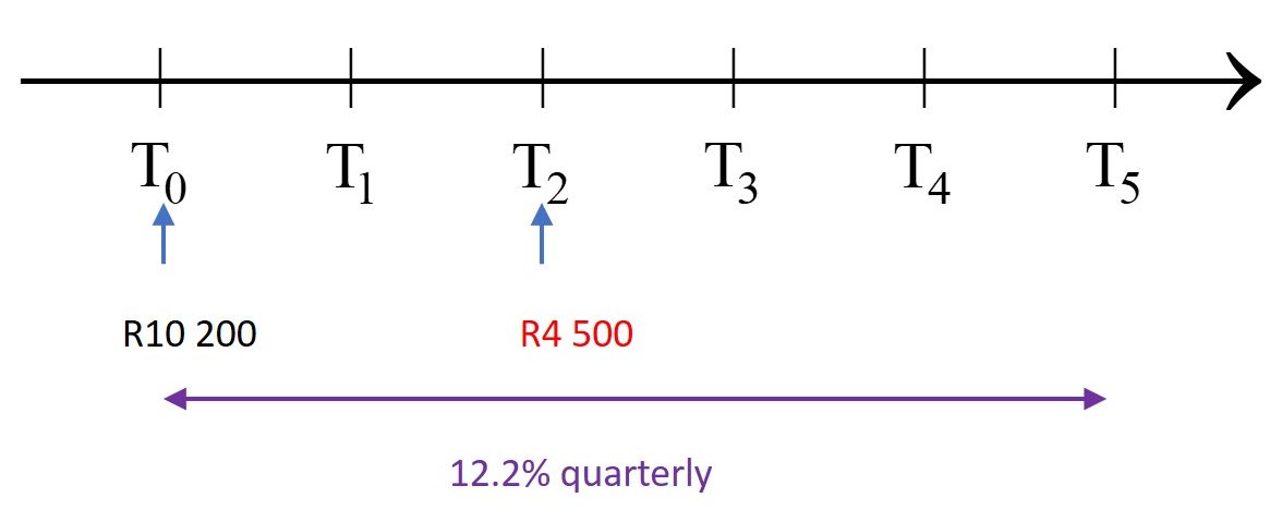
Consider the first period:
[latex]\scriptsize \begin{align*}{{A}_{1}}&={{P}_{1}}{{\left( {1+\displaystyle \frac{r}{{100\times m}}} \right)}^{{t\times m}}}\\&=10\text{ }200{{\left( {1+\displaystyle \frac{{12.2}}{{100\times 4}}} \right)}^{{2\times 4}}}\\&=10\text{ }200{{\left( {1.0305} \right)}^{8}}\end{align*}[/latex]
.
Consider the second period:
The principal at the start of the second period is [latex]\scriptsize \text{R}4\text{ 500}[/latex] less than the amount accumulated by the end of the first period.
[latex]\scriptsize \begin{align*}{{A}_{2}}&={{P}_{2}}{{\left( {1+\displaystyle \frac{r}{{100\times m}}} \right)}^{{t\times m}}}\\&=\left[ {10\text{ }200{{{\left( {1.0305} \right)}}^{8}}-4\text{ }500} \right]{{\left( {1.0305} \right)}^{{3\times 4}}}\\&=\left[ {12\text{ }971.31902-4\text{ }500} \right]{{\left( {1.0305} \right)}^{{12}}}\\&=12\text{ }148.62119\end{align*}[/latex]
At the end of five years there will be [latex]\scriptsize \text{R}12\text{ 148}\text{.62}[/latex] in the account.
Media Attributions
- M3 SO5.2 Unit3 Image1 Example 3.1 © DHET is licensed under a CC BY (Attribution) license
- M3 SO5.2 NOTE-calculator memory
- M3 SO5.2 Unit 3 Take Note RCL M+
- M3 SO5.2 Unit3 Image2 NOTE on calculator memory © DHET is licensed under a CC BY (Attribution) license
- M3 SO5.2 demonstrating calculator use
- M3 SO5.2 Unit3 Image3 NOTE2 on calculator memory © DHET is licensed under a CC BY (Attribution) license
- M3 SO5.2 Unit3 Image4 Example3.2 © DHET is licensed under a CC BY (Attribution) license
- M3 SO5.2 Unit3 Image5 Solution Ex3.1 No1a © DHET is licensed under a CC BY (Attribution) license
- M3 SO5.2 Unit3 Image6 Solution Ex3.1 No2 © DHET is licensed under a CC BY (Attribution) license
- M3 SO5.2 Unit3 Image7 Solution Ex3.1 No3 © DHET is licensed under a CC BY (Attribution) license
- M3 SO5.2 Unit3 Image8 Solution Ex3.1 No4 © DHET is licensed under a CC BY (Attribution) license
- M3 SO5.2 Unit3 Image9 Solution Ex3.1 No5 © DHET is licensed under a CC BY (Attribution) license
- M3 SO5.2 Unit3 Image10 Solution Ex3.1 No6 © DHET is licensed under a CC BY (Attribution) license
- M3 SO5.2 Unit3 Image11 Solution Assessment No1 © DHET is licensed under a CC BY (Attribution) license
- M3 SO5.2 Unit3 Image12 Solution Assessment No2 © DHET is licensed under a CC BY (Attribution) license
