Functions and algebra: Use a variety of techniques to sketch and interpret information from graphs of functions
Unit 10: Horizontal transformation of the cosine graph
Dylan Busa
Unit outcomes
By the end of this unit you will be able to:
- Sketch functions of the form [latex]\scriptsize y=\cos (\theta +p)[/latex].
- Determine the effects of positive and negative values of [latex]\scriptsize p[/latex] on the cosine graph [latex]\scriptsize y=\cos (\theta +p)[/latex].
- Find the value of [latex]\scriptsize p[/latex] from a given cosine graph of the form [latex]\scriptsize y=\cos (\theta +p)[/latex].
Remember that the domain of trigonometric functions can be represented as [latex]\scriptsize x[/latex] or [latex]\scriptsize \theta[/latex]. Therefore, [latex]\scriptsize y=\cos x[/latex] and [latex]\scriptsize y=\cos \theta[/latex] are the same function.
What you should know
Before you start this unit, make sure you can:
- Sketch cosine functions of the form [latex]\scriptsize y=a\cos \theta +q[/latex]. Refer to level 2 subject outcome 2.1 Unit 5 if you need help with this.
Introduction
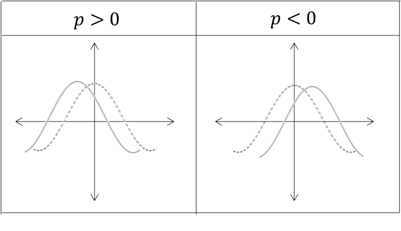
It should not surprise you that the effect of [latex]\scriptsize p[/latex] in [latex]\scriptsize y=\cos (x+p)[/latex] is to shift the graph horizontally by [latex]\scriptsize p[/latex] units. If [latex]\scriptsize p \gt 0[/latex], the graph is shifted [latex]\scriptsize p[/latex] units to the left. If [latex]\scriptsize p \lt 0[/latex], the graph is shifted [latex]\scriptsize p[/latex] units to the right.
Take note!
In [latex]\scriptsize y=\cos (x+p)[/latex]:
- if [latex]\scriptsize p \gt 0[/latex], the graph is shifted [latex]\scriptsize p[/latex] units to the left
- if [latex]\scriptsize p \lt 0[/latex], the graph is shifted [latex]\scriptsize p[/latex] units to the right.
Note
If you have an internet connection, spend some time playing with this interactive simulation.
Here you will find a graph of the function [latex]\scriptsize \displaystyle y=\cos (x+p)[/latex] with a slider to change the value of [latex]\scriptsize p[/latex]. Pay particular attention to how changing the value of [latex]\scriptsize p[/latex] affects the location of the turning points and the intercepts with the x-axis.
Sketch functions of the form [latex]\scriptsize y=\cos (x+p)[/latex]
The best way to sketch functions of the form [latex]\scriptsize y=\cos (x+p)[/latex] is to transform the basic function of [latex]\scriptsize y=\cos x[/latex] depending on the value of [latex]\scriptsize p[/latex]. To do this, you need to know the set of ‘anchor points’ of [latex]\scriptsize y=\cos x[/latex], as transformation of these points will help you to sketch functions of the form[latex]\scriptsize y=\cos (x+p)[/latex].
Example 10.1
Given the function [latex]\scriptsize y=\cos (x-{{30}^\circ})[/latex]:
- Sketch the function for the interval [latex]\scriptsize {{0}^\circ}\le x\le {{360}^\circ}[/latex].
- State the intercepts with the axes.
- State the domain and range.
- State the period.
- State the amplitude.
Solutions
- The function is of the form [latex]\scriptsize y=\cos (x+p)[/latex] with [latex]\scriptsize p=-{{30}^\circ}[/latex].
.
We need to transform one period of ‘anchor points’ noting that each of these points is going to be shifted [latex]\scriptsize {{30}^\circ}[/latex] to the right.
.[latex]\scriptsize \cos x[/latex] [latex]\scriptsize ({{0}^\circ},1)[/latex] [latex]\scriptsize ({{90}^\circ},0)[/latex] [latex]\scriptsize ({{180}^\circ},-1)[/latex] [latex]\scriptsize ({{270}^\circ},0)[/latex] [latex]\scriptsize ({{360}^\circ},1)[/latex] [latex]\scriptsize \cos (x-{{30}^\circ})[/latex] [latex]\scriptsize ({{30}^\circ},1)[/latex] [latex]\scriptsize ({{120}^\circ},0)[/latex] [latex]\scriptsize ({{210}^\circ},-1)[/latex] [latex]\scriptsize ({{300}^\circ},0)[/latex] [latex]\scriptsize ({{390}^\circ},1)[/latex] .
To make sure that the shape of the graph is as accurate as possible, we must also find the y-intercept.
y-intercept (let [latex]\scriptsize x=0[/latex]):
[latex]\scriptsize \begin{align*}y & =\cos ({{0}^\circ}-{{30}^\circ})\\\therefore y & =\displaystyle \frac{{\sqrt{3}}}{2}=0.866\end{align*}[/latex]
.
Because the period of the function is [latex]\scriptsize {{360}^\circ}[/latex] we know that the function value at [latex]\scriptsize {{360}^\circ}[/latex] will also be [latex]\scriptsize 0.866[/latex].
.
We can now plot our transformed ‘anchor points’ and draw the graph for the interval [latex]\scriptsize {{0}^\circ}\le x\le {{360}^\circ}[/latex].
.
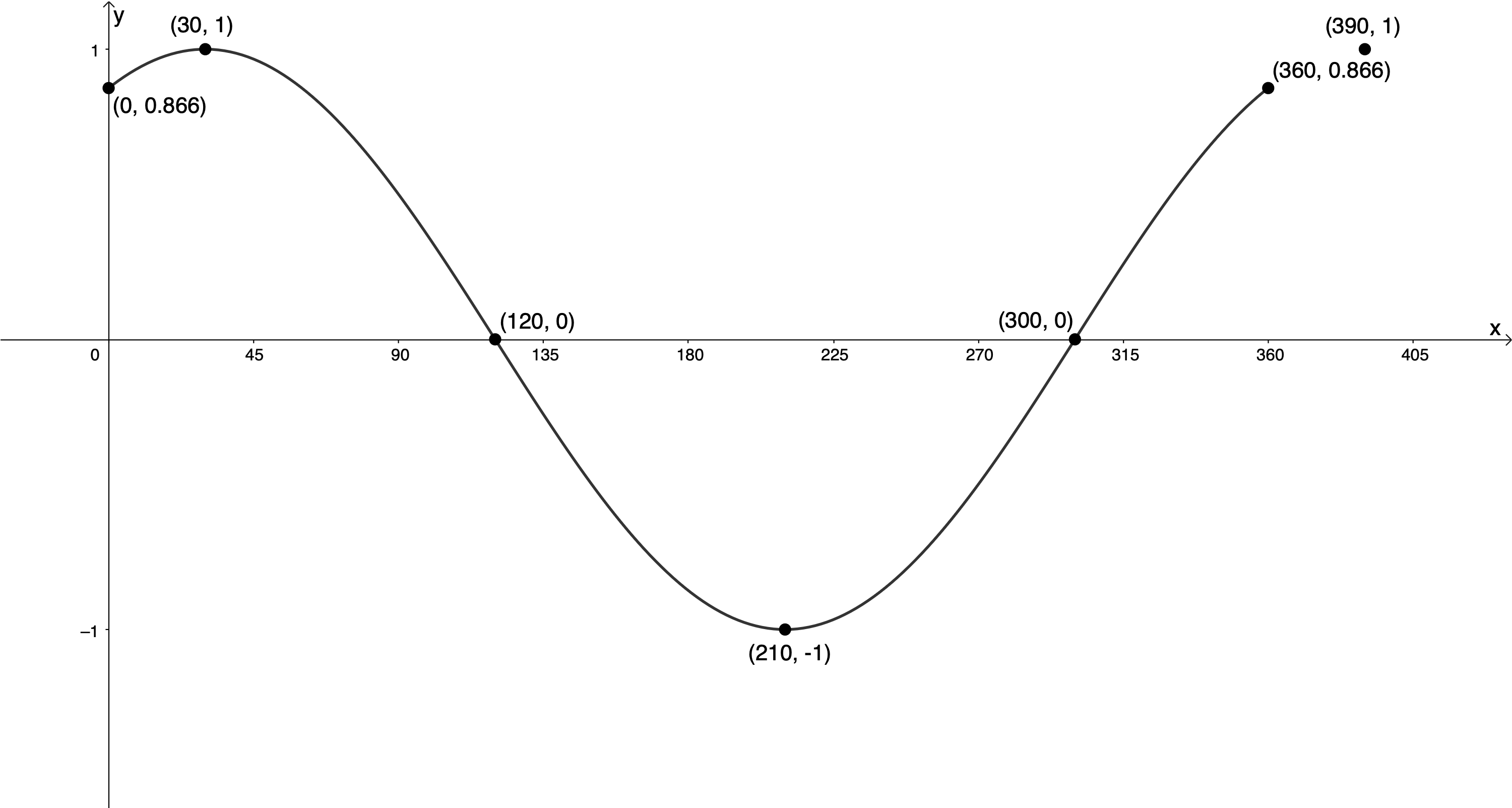
- y-intercept: [latex]\scriptsize ({{0}^\circ},0.866)[/latex]
x-intercepts: [latex]\scriptsize ({{120}^\circ},0)[/latex] and [latex]\scriptsize ({{300}^\circ},0)[/latex] - Domain: [latex]\scriptsize \{x|x\in \mathbb{R},\text{ }{{0}^\circ}\le x\le {{360}^\circ}\}[/latex]
Range: [latex]\scriptsize \{y|y\in \mathbb{R},\text{ }-1\le x\le 1\}[/latex] - The period is [latex]\scriptsize {{360}^\circ}[/latex].
- The amplitude is [latex]\scriptsize 1[/latex].
Take note!
In general, the domain of the function [latex]\scriptsize y=\cos (x+p)[/latex] is [latex]\scriptsize x\in \mathbb{R}\text{ }[/latex]. We had to restrict the domain in Example 10.1, because the interval in which we were working was restricted.
Exercise 10.1
Sketch the following functions for the indicated intervals on separate sets of axes:
- [latex]\scriptsize f(x)=\cos (x+{{30}^\circ})[/latex] for [latex]\scriptsize {{0}^\circ}\le x\le {{360}^\circ}[/latex]
- [latex]\scriptsize g(x)=\cos (x-{{45}^\circ})[/latex] for [latex]\scriptsize -{{360}^\circ}\le x\le {{360}^\circ}[/latex]
- [latex]\scriptsize h(x)=\cos (x-{{40}^\circ})[/latex] for [latex]\scriptsize -{{360}^\circ}\le x\le {{360}^\circ}[/latex]
The full solutions are at the end of the unit.
Sketch functions of the form [latex]\scriptsize y=a\cos (x+p)[/latex]
Now that we know that the value of [latex]\scriptsize p[/latex] shifts the function of the form [latex]\scriptsize y=\cos (x+p)[/latex] horizontally by [latex]\scriptsize p[/latex] degrees, we can combine this with our knowledge of the effects of [latex]\scriptsize a[/latex], and examine functions of the form [latex]\scriptsize y=a\cos (x+p)[/latex].
Example 10.2
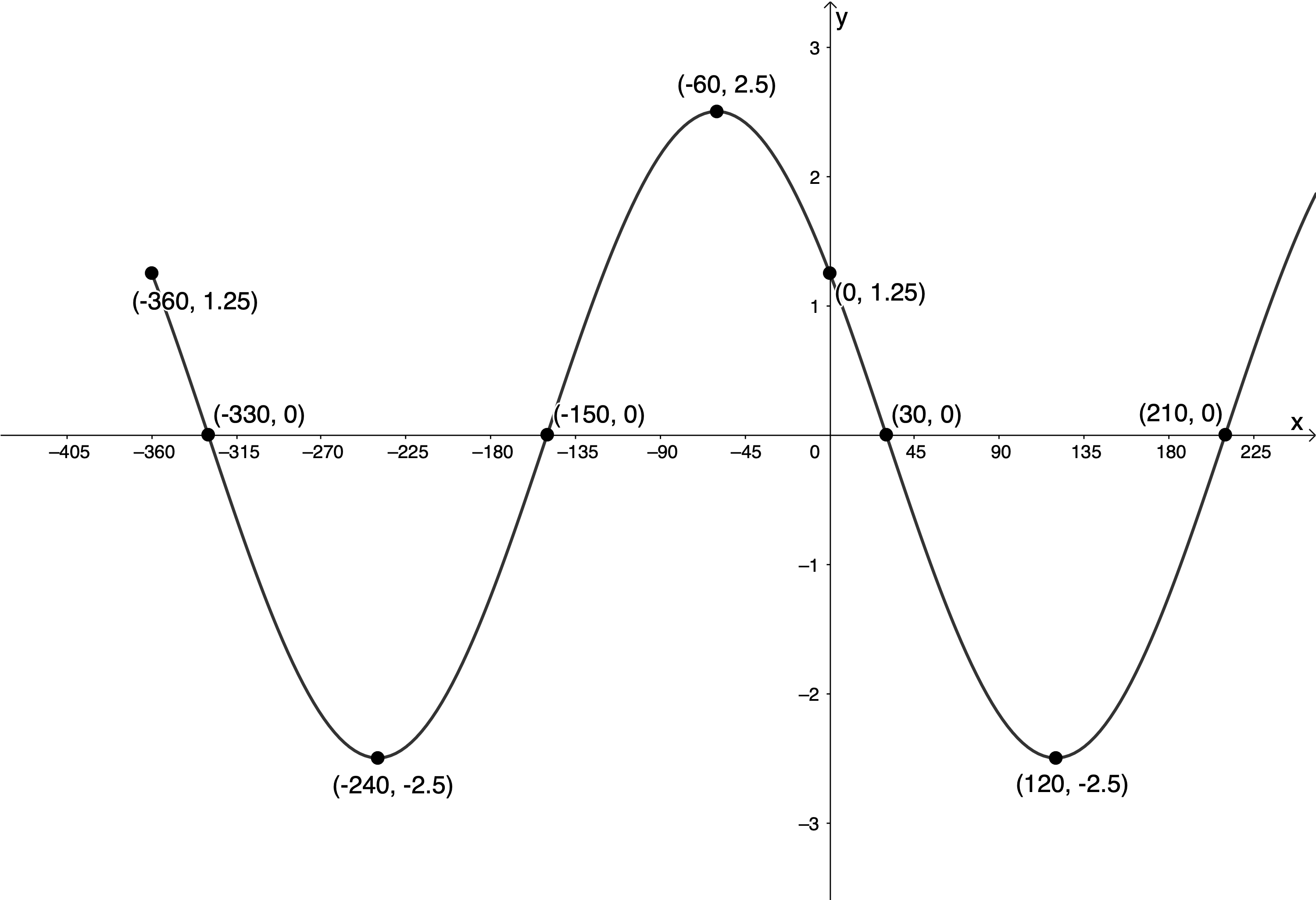
Sketch the graph of [latex]\scriptsize f(x)=2.5\cos (x+{{60}^\circ})[/latex] for the interval [latex]\scriptsize -{{360}^\circ}\le x\le {{360}^\circ}[/latex].
Solution
The function is of the form [latex]\scriptsize y=a\cos (x+p)[/latex] where [latex]\scriptsize a=2.5[/latex] and [latex]\scriptsize p={{60}^\circ}[/latex].
We need to transform one period of ‘anchor points’ noting that each of these points is going to be shifted [latex]\scriptsize {{60}^\circ}[/latex] to the left and each of the y-values is going to be multiplied by [latex]\scriptsize 2.5[/latex].
| [latex]\scriptsize \cos x[/latex] | [latex]\scriptsize ({{0}^\circ},1)[/latex] | [latex]\scriptsize ({{90}^\circ},0)[/latex] | [latex]\scriptsize ({{180}^\circ},-1)[/latex] | [latex]\scriptsize ({{270}^\circ},0)[/latex] | [latex]\scriptsize ({{360}^\circ},1)[/latex] |
| [latex]\scriptsize 2.5\cos (x+{{60}^\circ})[/latex] | [latex]\scriptsize (-{{60}^\circ},2.5)[/latex] | [latex]\scriptsize ({{30}^\circ},0)[/latex] | [latex]\scriptsize ({{120}^\circ},-2.5)[/latex] | [latex]\scriptsize ({{210}^\circ},0)[/latex] | [latex]\scriptsize ({{300}^\circ},2.5)[/latex] |
To make sure that the shape of the graph is as accurate as possible, we must also find the y-intercept.
y-intercept (let [latex]\scriptsize x=0[/latex]):
[latex]\scriptsize \begin{align*}y & =2.5\cos (0+{{60}^\circ})\\\therefore y & =2.5\times \displaystyle \frac{1}{2}\\=1.25\end{align*}[/latex]
Because the period of the function is [latex]\scriptsize {{360}^\circ}[/latex] we know that the function values at [latex]\scriptsize -{{360}^\circ}[/latex] and [latex]\scriptsize {{360}^\circ}[/latex] will also be [latex]\scriptsize 1.25[/latex].
We can now plot our transformed ‘anchor points’ and draw the graph for the interval [latex]\scriptsize -{{360}^\circ}\le x\le {{360}^\circ}[/latex].
Example 10.3
Given the function [latex]\scriptsize f(x)=2\cos ({{30}^\circ}-x)[/latex]:
- Sketch the graph for the interval [latex]\scriptsize {{0}^\circ}\le x\le {{360}^\circ}[/latex].
- State the intercepts with the axes.
- State the domain and range.
- State the amplitude and period.
Solutions
- The function is not in the form [latex]\scriptsize y=a\cos (x+p)[/latex]. We first need to get it into this form.
[latex]\scriptsize \begin{align*}f(x)&=2\cos ({{30}^\circ}-x)\\&=2\cos (-x+{{30}^\circ})\\&=2\cos \left( {-\left( {x-{{{30}}^\circ}} \right)} \right)\\&=2\cos (x-{{30}^\circ})\end{align*}[/latex]
.
Remember we learnt in unit 9 that [latex]\scriptsize \cos (-x)=\cos x[/latex] because the function is symmetrical about the y-axis and this meant that we get the same function value for [latex]\scriptsize -x[/latex] as we do for [latex]\scriptsize x[/latex]. This is why [latex]\scriptsize 2\cos \left( {-\left( {x-{{{30}}^\circ}} \right)} \right)=2\cos (x-{{30}^\circ})[/latex].
.
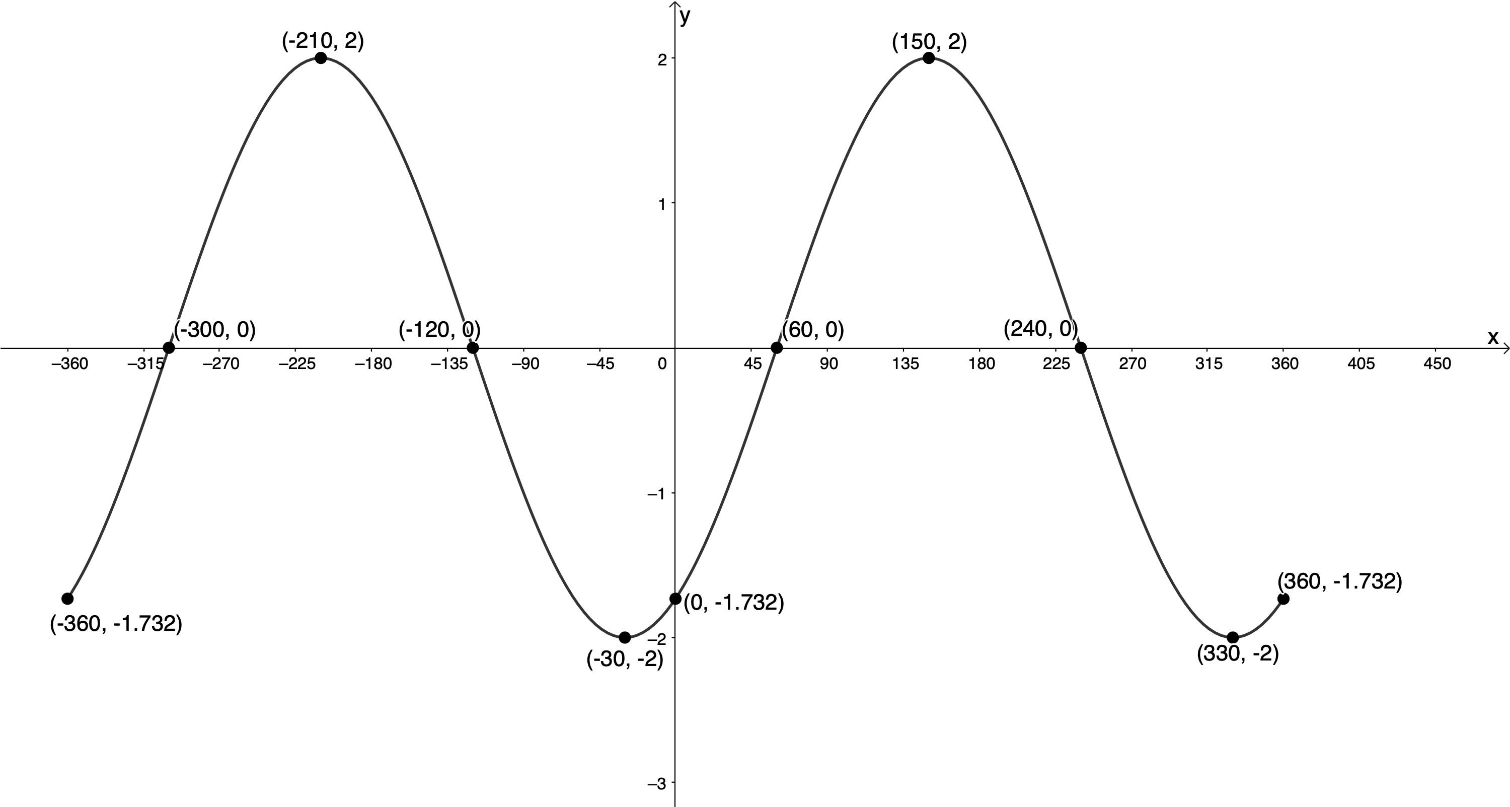
We need to transform one period of ‘anchor points’ noting that each of these points is going to be shifted [latex]\scriptsize {{30}^\circ}[/latex] to the right and each of the y-values of these points need to be multiplied by [latex]\scriptsize 2[/latex].
.[latex]\scriptsize \cos x[/latex] [latex]\scriptsize ({{0}^\circ},1)[/latex] [latex]\scriptsize ({{90}^\circ},0)[/latex] [latex]\scriptsize ({{180}^\circ},-1)[/latex] [latex]\scriptsize ({{270}^\circ},0)[/latex] [latex]\scriptsize ({{360}^\circ},1)[/latex] [latex]\scriptsize 2\cos (x-{{30}^\circ})[/latex] [latex]\scriptsize ({{30}^\circ},2)[/latex] [latex]\scriptsize ({{120}^\circ},0)[/latex] [latex]\scriptsize ({{210}^\circ},-2)[/latex] [latex]\scriptsize ({{300}^\circ},0)[/latex] [latex]\scriptsize ({{390}^\circ},2)[/latex]
.
To make sure that the shape of the graph is as accurate as possible, we must also find the y-intercept.
y-intercept (let [latex]\scriptsize x=0[/latex]):
[latex]\scriptsize \displaystyle \begin{align*}f(0) & =2\cos ({{0}^\circ}-{{30}^\circ})\\\therefore f(0) & =2\times \displaystyle \frac{{\sqrt{3}}}{2}=\sqrt{3}=1.732\text{ }\end{align*}[/latex]
.
Because the period of the function is [latex]\scriptsize {{360}^\circ}[/latex] we know that the function value at [latex]\scriptsize {{360}^\circ}[/latex] will also be [latex]\scriptsize 1.732[/latex].
.
We can now plot our transformed ‘anchor points’ and draw the graph for the interval [latex]\scriptsize {{0}^\circ}\le x\le {{360}^\circ}[/latex].
.
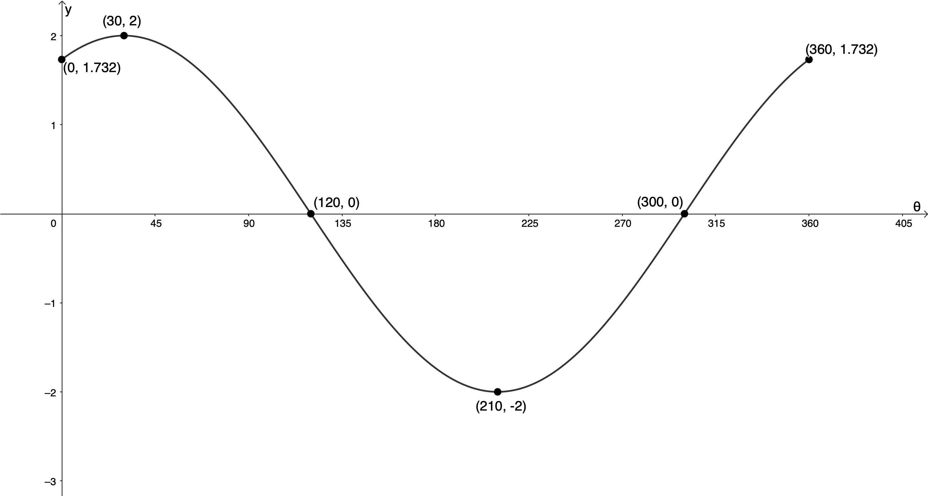
- y-intercept: [latex]\scriptsize ({{0}^\circ},\sqrt{3})[/latex] or [latex]\scriptsize ({{0}^\circ},1.732)[/latex]
x-intercepts: [latex]\scriptsize ({{120}^\circ},0)[/latex] and [latex]\scriptsize ({{300}^\circ},0)[/latex] - Domain: [latex]\scriptsize \{x|x\in \mathbb{R},\text{ }{{0}^\circ}\le x\le {{360}^\circ}\}[/latex]
Range: [latex]\scriptsize \{f(x)|f(x)\in \mathbb{R},\text{ }-2\le f(x)\le 2\}[/latex] - The period is [latex]\scriptsize {{360}^\circ}[/latex].
The amplitude is [latex]\scriptsize 2[/latex].
Exercise 10.2
For each of the following functions, sketch the graph for the indicated interval and state the domain and range and intercepts with the axes:
- [latex]\scriptsize y=-2\cos (x+{{30}^\circ})[/latex] for [latex]\scriptsize -{{360}^\circ}\le x\le {{360}^\circ}[/latex]
- [latex]\scriptsize 2y=\cos (x+{{60}^\circ})[/latex] for [latex]\scriptsize {{0}^\circ}\le x\le {{360}^\circ}[/latex]
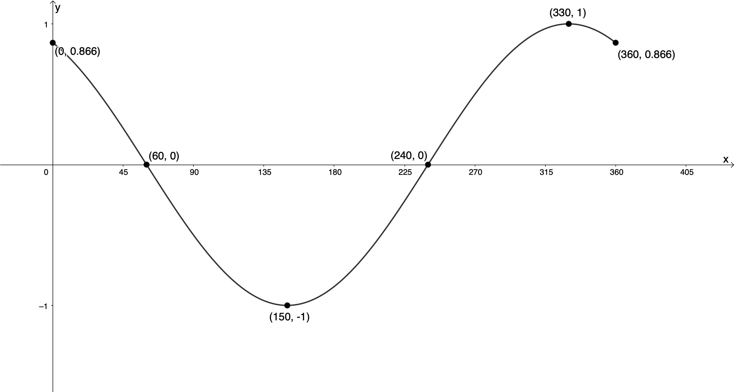
- [latex]\scriptsize \displaystyle \frac{1}{3}y=\cos ({{60}^\circ}-x)[/latex] for [latex]\scriptsize -{{360}^\circ}\le x\le {{360}^\circ}[/latex]
The full solutions are at the end of the unit.
Find the equation of a cosine function of the form [latex]\scriptsize y=a\cos (x+p)[/latex]
By examining the amplitude and the horizontal shift of [latex]\scriptsize y=a\cos (x+p)[/latex], we can determine the values of [latex]\scriptsize a[/latex] and [latex]\scriptsize p[/latex].
Example 10.4
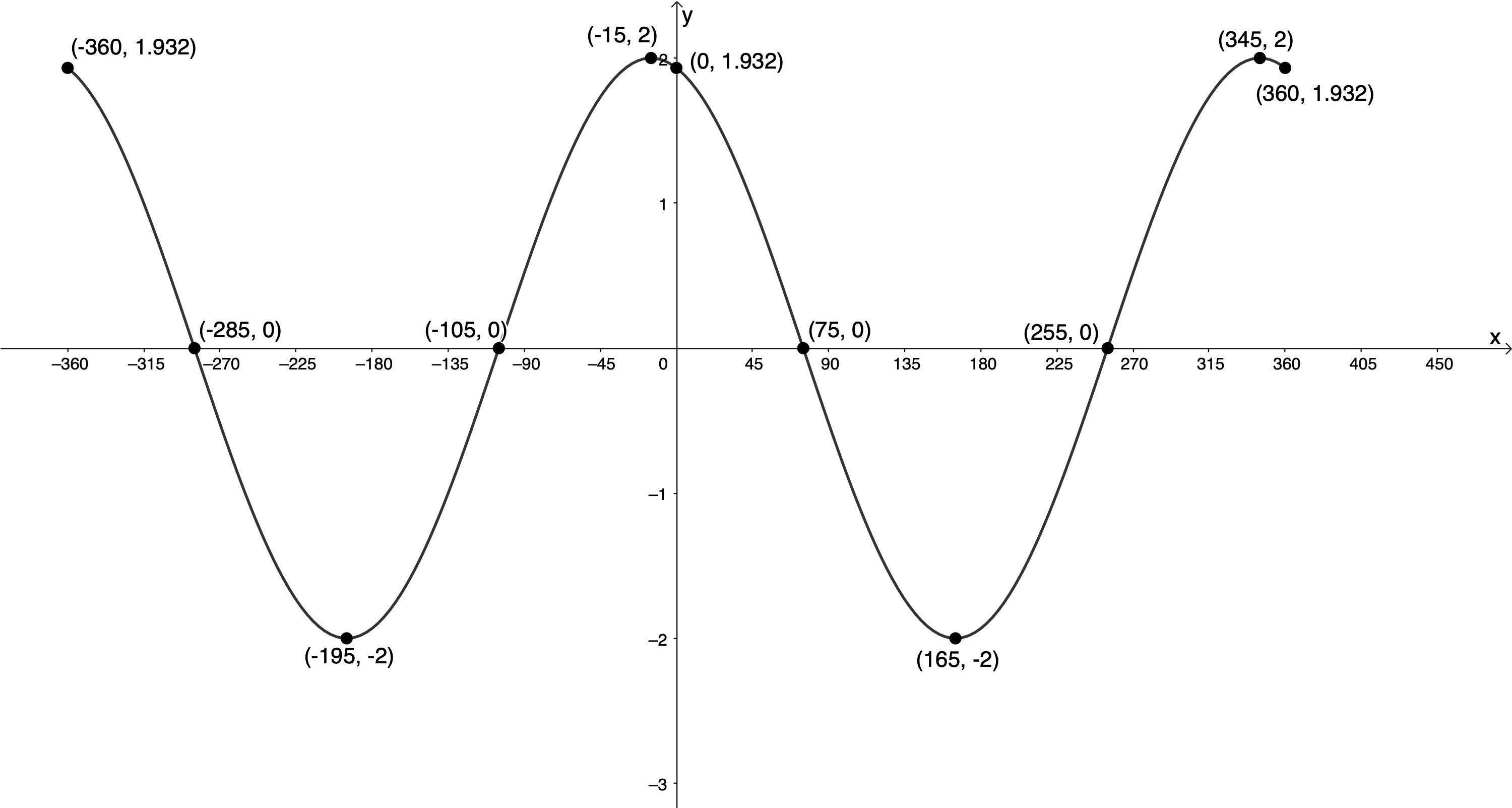
The graph below is a function of the form [latex]\scriptsize y=a\cos (x+p)[/latex]. Determine the values of [latex]\scriptsize a[/latex] and [latex]\scriptsize p[/latex].
Solution
We are told that the function is of the form [latex]\scriptsize y=a\cos (x+p)[/latex].
Firstly, we can see that the amplitude of the graph is [latex]\scriptsize 2[/latex] units. We do not yet know whether [latex]\scriptsize a=2[/latex] or [latex]\scriptsize a=-2[/latex].
We know that the function [latex]\scriptsize y=\cos x[/latex] has a maximum turning point at [latex]\scriptsize ({{0}^\circ},1)[/latex]. The function above has a maximum turning point at [latex]\scriptsize (-{{15}^\circ},2)[/latex]. Therefore, the function has been shifted [latex]\scriptsize {{15}^\circ}[/latex] to the left and [latex]\scriptsize p={{15}^\circ}[/latex].
The amplitude of the graph is [latex]\scriptsize 2[/latex] and has not been reflected about the x-axis. Therefore, [latex]\scriptsize a=2[/latex].
The function is [latex]\scriptsize y=2\cos (x+{{15}^\circ})[/latex].
Example 10.5
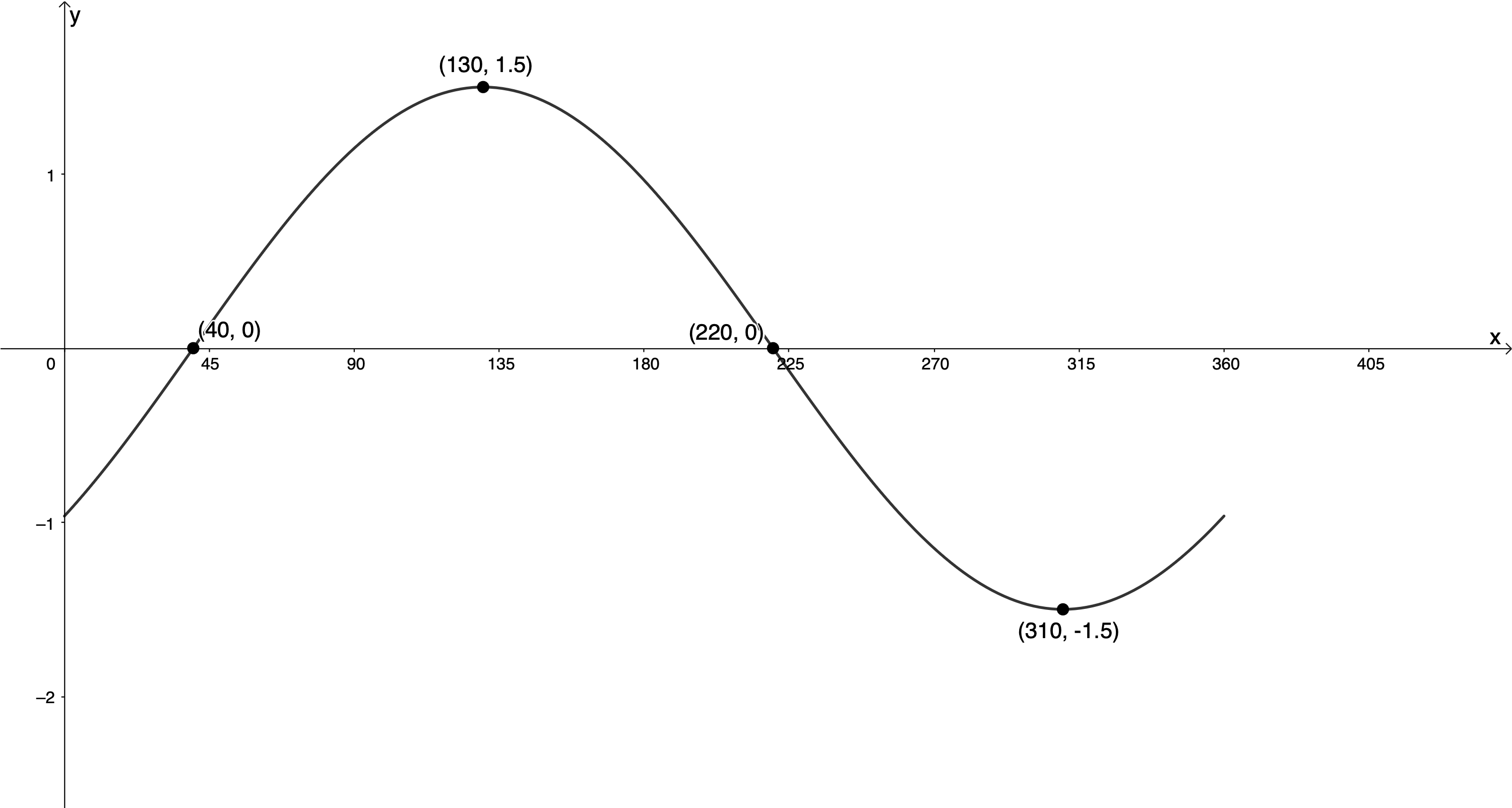
The graph below is a function of the form [latex]\scriptsize y=a\cos (x+p)[/latex]. Determine the values of [latex]\scriptsize a[/latex] and [latex]\scriptsize p[/latex].
Solution
We are told that the function is of the form [latex]\scriptsize y=a\cos (x+p)[/latex].
Firstly, we can see that the amplitude of the graph is [latex]\scriptsize 1.5[/latex] units. We do not yet know whether [latex]\scriptsize a=1.5[/latex] or [latex]\scriptsize a=-1.5[/latex].
We know that the function [latex]\scriptsize y=\cos x[/latex] has a maximum turning point at [latex]\scriptsize ({{0}^\circ},1)[/latex] and then cuts the x-axis at [latex]\scriptsize ({{90}^\circ},0)[/latex]. This function instead has a maximum turning point at [latex]\scriptsize ({{130}^\circ},1.5)[/latex]. Therefore, we can say that the point [latex]\scriptsize ({{0}^\circ},1)[/latex] has been transformed into the point [latex]\scriptsize ({{130}^\circ},1.5)[/latex]. This would indicate that that graph has been shifted [latex]\scriptsize {{130}^\circ}[/latex] to the right and therefore that[latex]\scriptsize p=-{{130}^\circ}[/latex].
However, we generally prefer [latex]\scriptsize -{{90}^\circ}\le p\le {{90}^\circ}[/latex]. We also know that the function [latex]\scriptsize y=\cos x[/latex] has a minimum turning point at [latex]\scriptsize ({{180}^\circ},-1)[/latex]. Therefore, we can also say that the point [latex]\scriptsize ({{130}^\circ},1.5)[/latex] is the result of a [latex]\scriptsize {{50}^\circ}[/latex] shift to the left and that the function has been reflected about the x-axis. Because this gives us a value for [latex]\scriptsize p[/latex] that is [latex]\scriptsize -{{90}^\circ}\le p\le {{90}^\circ}[/latex], this is the transformation we will use.
This means that [latex]\scriptsize p={{50}^\circ}[/latex], [latex]\scriptsize a=-1.5[/latex] and that the function is [latex]\scriptsize y=-1.5\cos (x+{{50}^\circ})[/latex].
Exercise 10.3
Given the graph of the form [latex]\scriptsize y=a\cos (x+p)[/latex]:
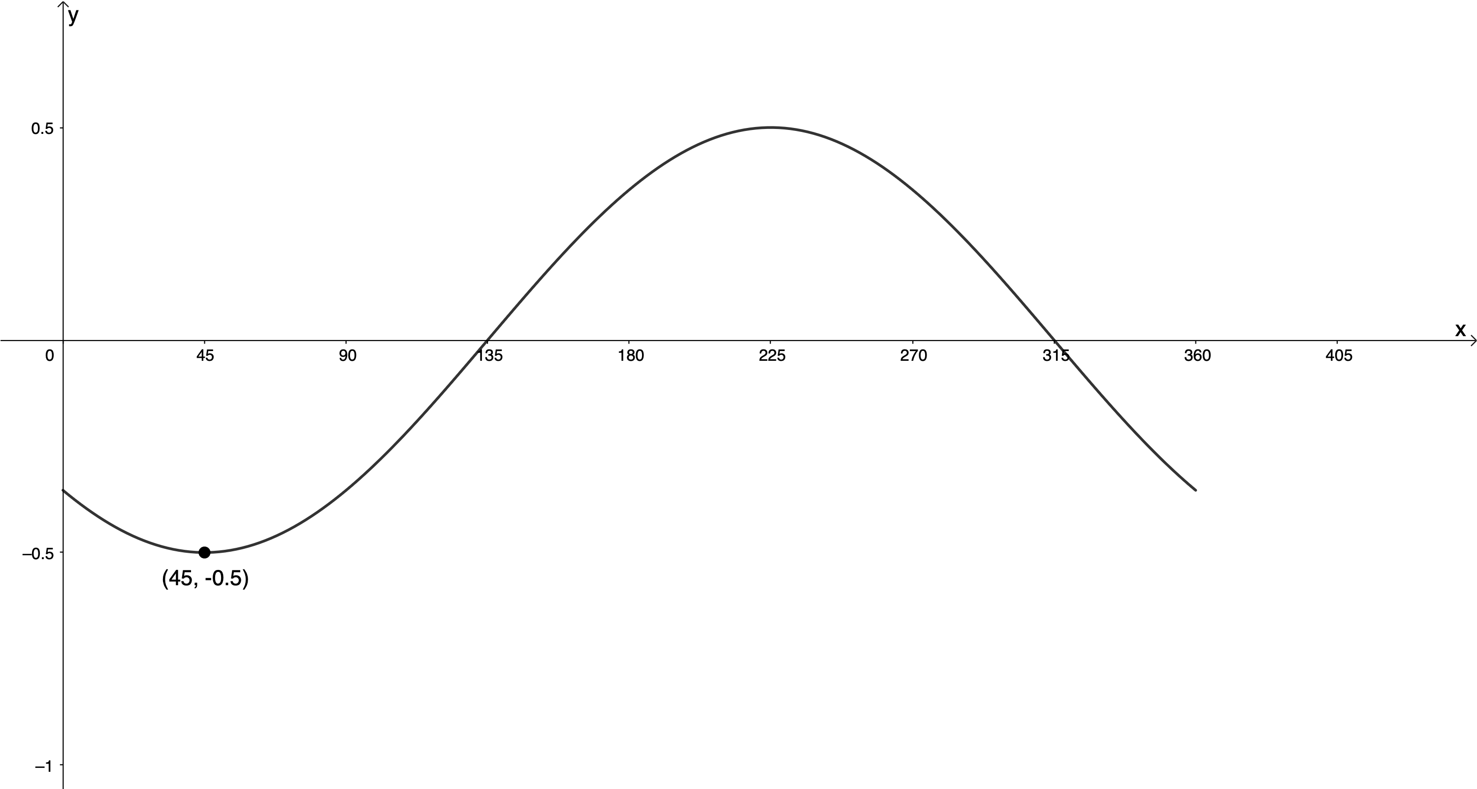
- Determine the values of [latex]\scriptsize a[/latex] and [latex]\scriptsize p[/latex].
- State the domain and range of the function.
The full solutions are at the end of the unit.
The relationship between [latex]\scriptsize y=\sin x[/latex] and [latex]\scriptsize y=\cos x[/latex]
You may have noticed that the names of the functions sine and cosine are similar. Well, there is a very good reason for this as we will discover in Activity 10.1.
Activity 10.1: Co-functions
Time required: 20 minutes
What you need:
- a pen or pencil
- a calculator
- several pieces of paper
What to do:
- Consider the function [latex]\scriptsize f(x)=\cos (x-{{90}^\circ})[/latex]. Make a neat sketch of the graph of this function for the interval [latex]\scriptsize {{0}^\circ}\le x\le {{360}^\circ}[/latex] on a piece of paper. Use the following table of ‘anchor points’ to help you.
[latex]\scriptsize \cos x[/latex] [latex]\scriptsize ({{0}^\circ},1)[/latex] [latex]\scriptsize ({{90}^\circ},0)[/latex] [latex]\scriptsize ({{180}^\circ},-1)[/latex] [latex]\scriptsize ({{270}^\circ},0)[/latex] [latex]\scriptsize ({{360}^\circ},1)[/latex] [latex]\scriptsize \cos (x-{{90}^\circ})[/latex] - What do you notice about the graph of the function [latex]\scriptsize f(x)=\cos (x-{{90}^\circ})[/latex] and the function [latex]\scriptsize y=\sin x[/latex]?
- Write a mathematical expression that captures this relationship.
- Now consider the function [latex]\scriptsize g(x)=\sin (x-{{90}^\circ})[/latex]. Make a neat sketch of the graph of this function [latex]\scriptsize {{0}^\circ}\le x\le {{360}^\circ}[/latex] on a new piece of paper. Use the following table of ‘anchor points’ to help you.
[latex]\scriptsize \sin x[/latex] [latex]\scriptsize ({{0}^\circ},0)[/latex] [latex]\scriptsize ({{90}^\circ},1)[/latex] [latex]\scriptsize ({{180}^\circ},0)[/latex] [latex]\scriptsize ({{270}^\circ},-1)[/latex] [latex]\scriptsize ({{360}^\circ},0)[/latex] [latex]\scriptsize \sin (x-{{90}^\circ})[/latex] - What do you notice about the graph of the function [latex]\scriptsize g(x)=\sin (x-{{90}^\circ})[/latex] and the function [latex]\scriptsize y=\cos x[/latex]?
- Write a mathematical expression that captures this relationship.
- Do these relationships between the sine and cosine functions hold for [latex]\scriptsize y=\cos (x+{{90}^\circ})[/latex] and [latex]\scriptsize y=\sin (x+{{90}^\circ})[/latex]? Draw the graphs of these functions to help you.
What did you find?
- Here is the completed table of values. The graph of [latex]\scriptsize f(x)=\cos (x-{{90}^\circ})[/latex] for the interval [latex]\scriptsize {{0}^\circ}\le x\le {{360}^\circ}[/latex] is shown in Figure 7.
[latex]\scriptsize \cos x[/latex] [latex]\scriptsize ({{0}^\circ},1)[/latex] [latex]\scriptsize ({{90}^\circ},0)[/latex] [latex]\scriptsize ({{180}^\circ},-1)[/latex] [latex]\scriptsize ({{270}^\circ},0)[/latex] [latex]\scriptsize ({{360}^\circ},1)[/latex] [latex]\scriptsize \cos (x-{{90}^\circ})[/latex] [latex]\scriptsize ({{90}^\circ},1)[/latex] [latex]\scriptsize ({{180}^\circ},0)[/latex] [latex]\scriptsize ({{270}^\circ},-1)[/latex] [latex]\scriptsize ({{360}^\circ},0)[/latex] [latex]\scriptsize ({{450}^\circ},1)[/latex] 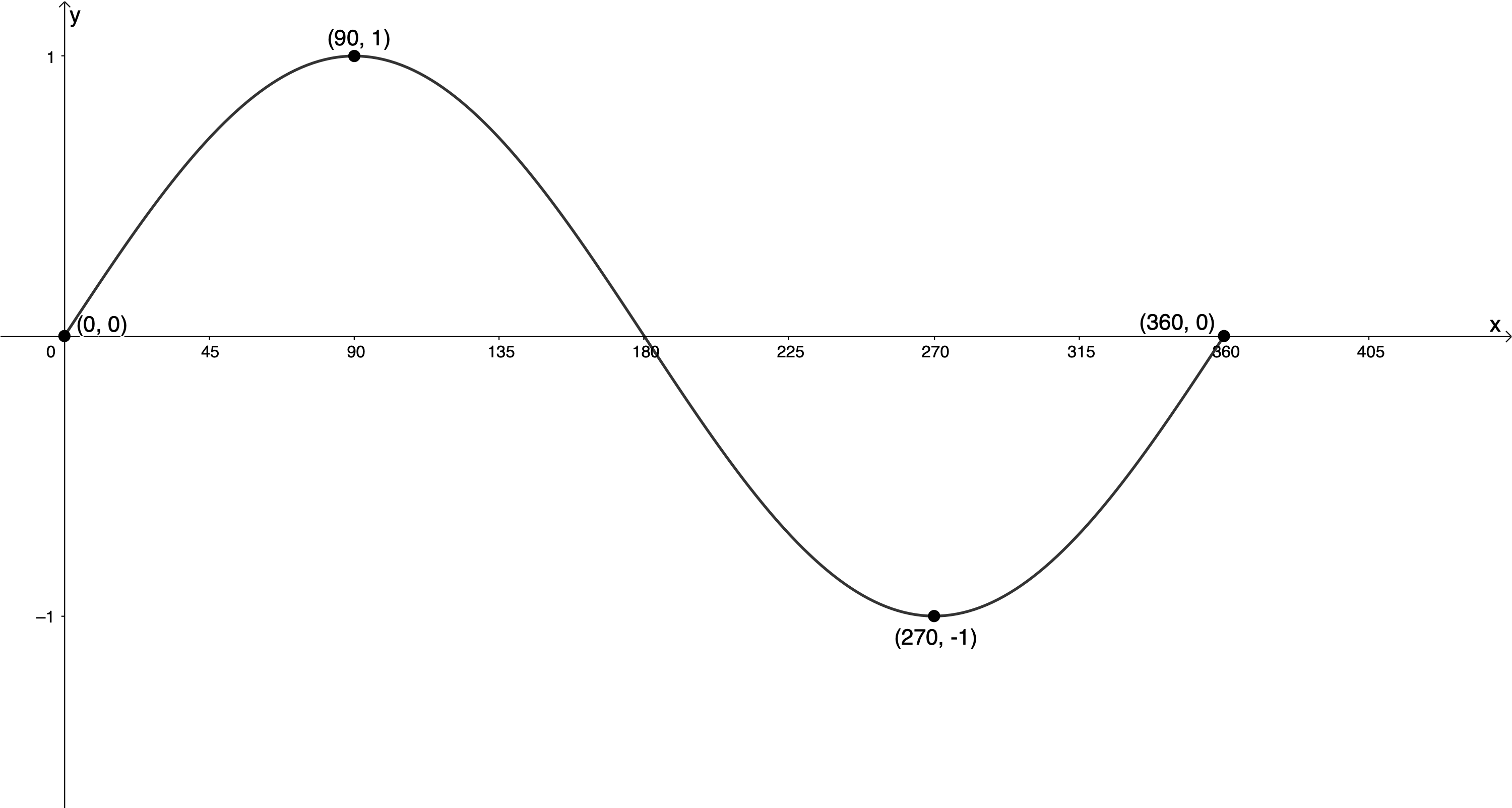
Figure 7: Graph of [latex]\scriptsize f(x)=\cos (x-{{90}^\circ})[/latex] - The graph of [latex]\scriptsize f(x)=\cos (x-{{90}^\circ})[/latex] is the same as the graph of [latex]\scriptsize y=\sin x[/latex].
- [latex]\scriptsize \cos (x-{{90}^\circ})=\sin x[/latex]
- Here is the completed table of values. The graph of [latex]\scriptsize g(x)=\sin (x-{{90}^\circ})[/latex] for the interval [latex]\scriptsize {{0}^\circ}\le x\le {{360}^\circ}[/latex] is shown in Figure 8.
[latex]\scriptsize \sin x[/latex] [latex]\scriptsize ({{0}^\circ},0)[/latex] [latex]\scriptsize ({{90}^\circ},1)[/latex] [latex]\scriptsize ({{180}^\circ},0)[/latex] [latex]\scriptsize ({{270}^\circ},-1)[/latex] [latex]\scriptsize ({{360}^\circ},0)[/latex] [latex]\scriptsize \sin (x-{{90}^\circ})[/latex] [latex]\scriptsize ({{90}^\circ},0)[/latex] [latex]\scriptsize ({{180}^\circ},1)[/latex] [latex]\scriptsize ({{270}^\circ},0)[/latex] [latex]\scriptsize ({{360}^\circ},-1)[/latex] [latex]\scriptsize ({{450}^\circ},0)[/latex] 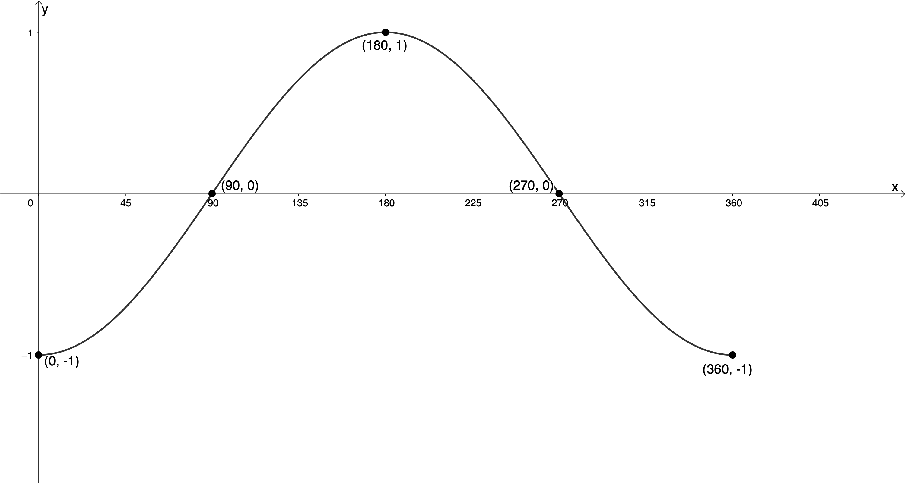
Figure 8: Graph of [latex]\scriptsize f(x)=\sin (x-{{90}^\circ})[/latex] - The graph of [latex]\scriptsize g(x)=\sin (x-{{90}^\circ})[/latex] is the same as the graph of [latex]\scriptsize y=-\cos x[/latex].
- [latex]\scriptsize \sin (x-{{90}^\circ})=-\cos x[/latex]
- If we sketch the function [latex]\scriptsize y=\cos (x+{{90}^\circ})[/latex] we get the graph in Figure 9. We can see that this is the same as the graph of [latex]\scriptsize y=-\sin x[/latex]. Therefore, [latex]\scriptsize \cos (x+{{90}^\circ})=-\sin x[/latex].
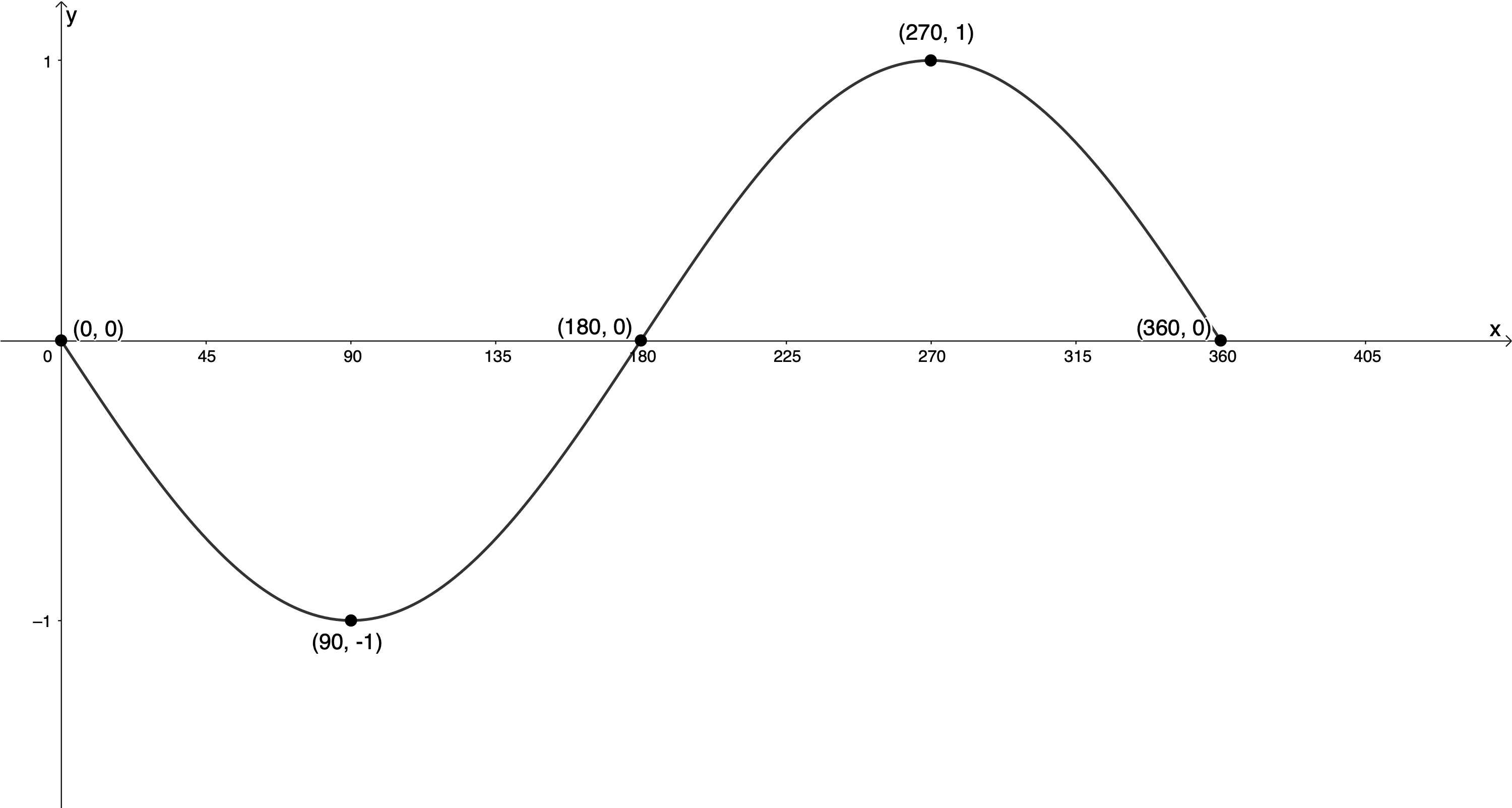
Figure 9: Graph of [latex]\scriptsize y=\cos (x+{{90}^\circ})[/latex] .
If we sketch the function [latex]\scriptsize y=\sin (x+{{90}^\circ})[/latex] we get the graph in Figure 10. We can see that this is the graph of [latex]\scriptsize y=\cos x[/latex]. Therefore, [latex]\scriptsize \sin (x+{{90}^\circ})=\cos x[/latex].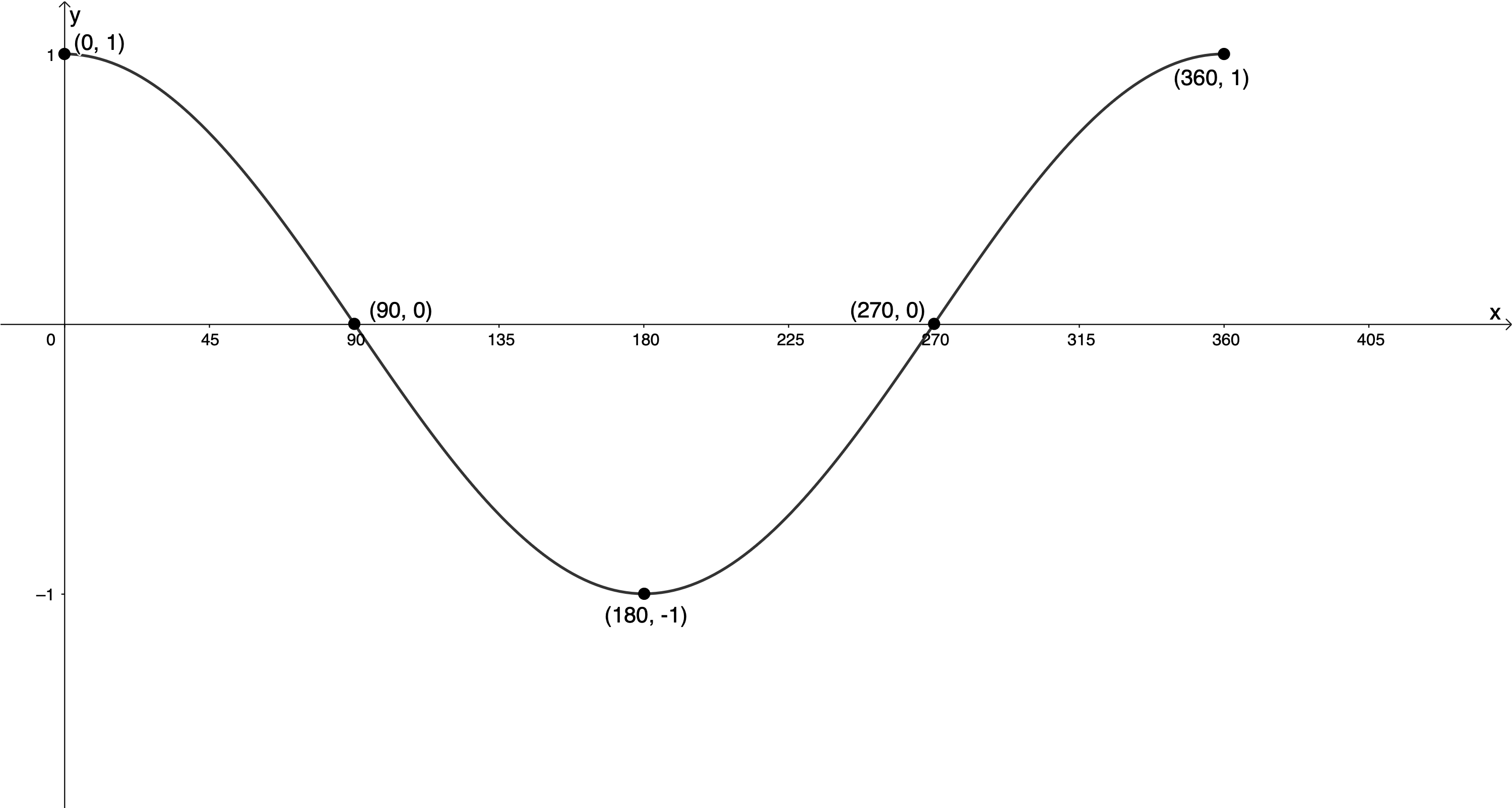
Figure 10: Graph of [latex]\scriptsize y=\sin (x+{{90}^\circ})[/latex]
In Activity 10.1 we learnt of the following relationships between the sine and cosine functions:
- [latex]\scriptsize \cos (x-{{90}^\circ})=\sin x[/latex]
- [latex]\scriptsize \sin (x-{{90}^\circ})=-\cos x[/latex]
- [latex]\scriptsize \cos (x+{{90}^\circ})=-\sin x[/latex]
- [latex]\scriptsize \sin (x+{{90}^\circ})=\cos x[/latex].
These relationships between the sine and cosine functions are precisely the reason for their names. We say that cosine is the co-function of sine because we can change one function into the other by adding or subtracting [latex]\scriptsize {{90}^\circ}[/latex] from the function input values. The reason for the change in signs has to do with whether the original function value is positive or negative.
Take [latex]\scriptsize \cos (x-{{90}^\circ})[/latex] for example. If we assume that [latex]\scriptsize x[/latex] is an acute angle ([latex]\scriptsize {{0}^\circ} \lt x \lt {{90}^\circ}[/latex]), then [latex]\scriptsize (x-{{90}^\circ})[/latex] will lie in the fourth quadrant where cosine is positive (see Figure 11). Therefore, because [latex]\scriptsize \cos (x-{{90}^\circ})[/latex]is positive, it is equal to [latex]\scriptsize \sin x[/latex] [latex]\scriptsize \cos (x-{{90}^\circ})=\sin x[/latex].
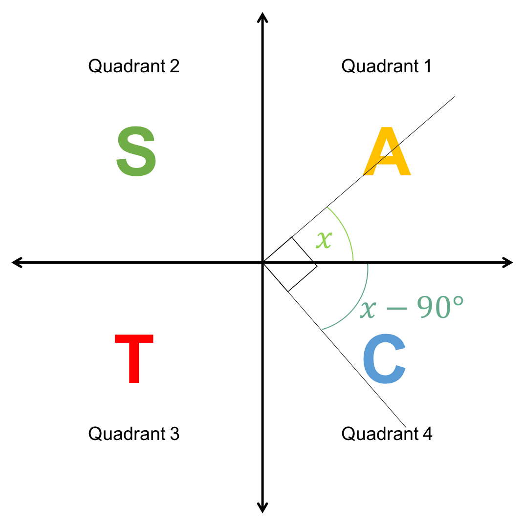
However, if we take [latex]\scriptsize \sin (x-{{90}^\circ})[/latex] and still assume that [latex]\scriptsize {{0}^\circ} \lt x \lt {{90}^\circ}[/latex], then [latex]\scriptsize (x-{{90}^\circ})[/latex] will still lie in the fourth quadrant where sine is negative. Therefore, we need the negative value of [latex]\scriptsize \cos x[/latex] to ensure that the ratios are still the same [latex]\scriptsize \sin (x-{{90}^\circ})=-\cos x[/latex].
Did you know?
The co-function of tangent is called cotangent or COT for short. Where [latex]\scriptsize \tan \theta =\displaystyle \frac{y}{x}[/latex] on the Cartesian plane, [latex]\scriptsize \cot \theta =\displaystyle \frac{x}{y}[/latex].
Summary
In this unit you have learnt the following:
- The effects of [latex]\scriptsize a[/latex] and [latex]\scriptsize p[/latex] on the cosine graph of the form [latex]\scriptsize y=a\cos (x+p)[/latex].
- How to sketch functions of the form [latex]\scriptsize y=a\cos (x+p)[/latex].
- How to find the values of [latex]\scriptsize a[/latex] and [latex]\scriptsize p[/latex] from a given cosine graph of the form [latex]\scriptsize y=a\cos (x+p)[/latex].
- That sine and cosine are co-functions, and that:
- [latex]\scriptsize \cos (x-{{90}^\circ})=\sin x[/latex]
- [latex]\scriptsize \sin (x-{{90}^\circ})=-\cos x[/latex]
- [latex]\scriptsize \cos (x+{{90}^\circ})=-\sin x[/latex]
- [latex]\scriptsize \sin (x+{{90}^\circ})=\cos x[/latex].
Unit 10: Assessment
Suggested time to complete: 55 minutes
- Sketch the following functions for the given intervals:
- [latex]\scriptsize 4y=\cos (x-{{60}^\circ})[/latex] for [latex]\scriptsize {{0}^\circ}\le x\le {{360}^\circ}[/latex]
- [latex]\scriptsize g(x)=-4\cos ({{45}^\circ}-x)[/latex] for [latex]\scriptsize -{{360}^\circ}\le x\le {{360}^\circ}[/latex]
- From the graph below of the form [latex]\scriptsize y=a\cos (x+p)[/latex], determine the values of [latex]\scriptsize a[/latex] and [latex]\scriptsize p[/latex].
- Given the following graph:
- Write the equation of this function in the form [latex]\scriptsize y=a\cos x[/latex].
- Write the equation of this function in the form [latex]\scriptsize y=\cos (x+p)[/latex].
- Write the equation of this function in the form [latex]\scriptsize y=\sin (x+p)[/latex].
The full solutions are at the end of the unit.
Unit 10: Solutions
Exercise 10.1
- [latex]\scriptsize f(x)=\cos (x+{{30}^\circ})[/latex] for [latex]\scriptsize {{0}^\circ}\le x\le {{360}^\circ}[/latex]
[latex]\scriptsize p={{30}^\circ}[/latex]. Therefore, the graph will be shifted [latex]\scriptsize {{30}^\circ}[/latex] to the left.[latex]\scriptsize \cos x[/latex] [latex]\scriptsize ({{0}^\circ},1)[/latex] [latex]\scriptsize ({{90}^\circ},0)[/latex] [latex]\scriptsize ({{180}^\circ},-1)[/latex] [latex]\scriptsize ({{270}^\circ},0)[/latex] [latex]\scriptsize ({{360}^\circ},1)[/latex] [latex]\scriptsize \cos (x+{{30}^\circ})[/latex] [latex]\scriptsize (-{{30}^\circ},1)[/latex] [latex]\scriptsize ({{60}^\circ},0)[/latex] [latex]\scriptsize ({{150}^\circ},-1)[/latex] [latex]\scriptsize ({{240}^\circ},0)[/latex] [latex]\scriptsize ({{330}^\circ},1)[/latex] .
y-intercept (let [latex]\scriptsize x=0[/latex]):
[latex]\scriptsize \begin{align*}f(0) & =\cos ({{0}^\circ}+{{30}^\circ})\\\therefore f(0) & =\displaystyle \frac{{\sqrt{3}}}{2}=0.866\text{ }\end{align*}[/latex]
.
Because the period of the function is [latex]\scriptsize {{360}^\circ}[/latex] we know that the function value at [latex]\scriptsize {{360}^\circ}[/latex] will also be [latex]\scriptsize 0.866[/latex].
.
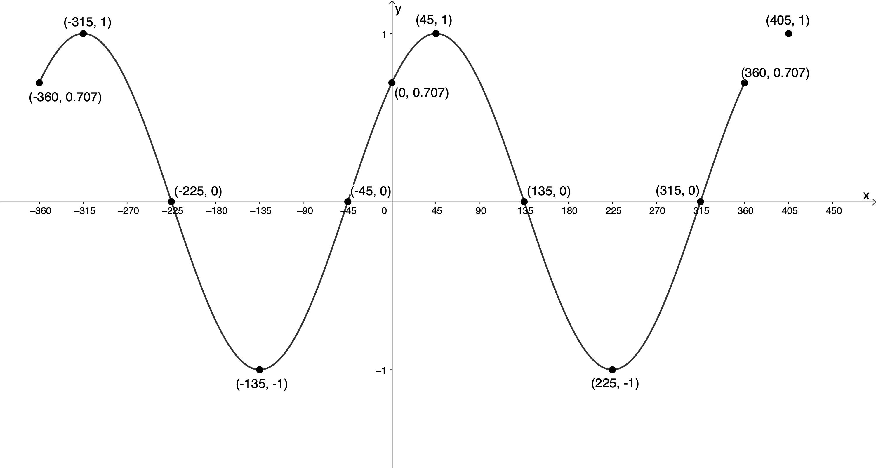
- [latex]\scriptsize g(x)=\cos (x-{{45}^\circ})[/latex] for [latex]\scriptsize -{{360}^\circ}\le x\le {{360}^\circ}[/latex]
[latex]\scriptsize p=-{{45}^\circ}[/latex]. Therefore, the graph will be shifted [latex]\scriptsize {{45}^\circ}[/latex] to the right.[latex]\scriptsize \cos x[/latex] [latex]\scriptsize ({{0}^\circ},1)[/latex] [latex]\scriptsize ({{90}^\circ},0)[/latex] [latex]\scriptsize ({{180}^\circ},-1)[/latex] [latex]\scriptsize ({{270}^\circ},0)[/latex] [latex]\scriptsize ({{360}^\circ},1)[/latex] [latex]\scriptsize \cos (x-{{45}^\circ})[/latex] [latex]\scriptsize ({{45}^\circ},1)[/latex] [latex]\scriptsize ({{135}^\circ},0)[/latex] [latex]\scriptsize ({{225}^\circ},-1)[/latex] [latex]\scriptsize ({{315}^\circ},0)[/latex] [latex]\scriptsize ({{405}^\circ},1)[/latex] .
y-intercept (let [latex]\scriptsize x=0[/latex]):
[latex]\scriptsize \begin{align*}g(0) & =\cos ({{0}^\circ}-{{45}^\circ})\\\therefore g(0) & =\displaystyle \frac{1}{{\sqrt{2}}}=0.707\end{align*}[/latex]
.
Because the period of the function is [latex]\scriptsize {{360}^\circ}[/latex] we know that the function values at [latex]\scriptsize -{{360}^\circ}[/latex] and [latex]\scriptsize {{360}^\circ}[/latex] will also be [latex]\scriptsize 0.707[/latex].
.
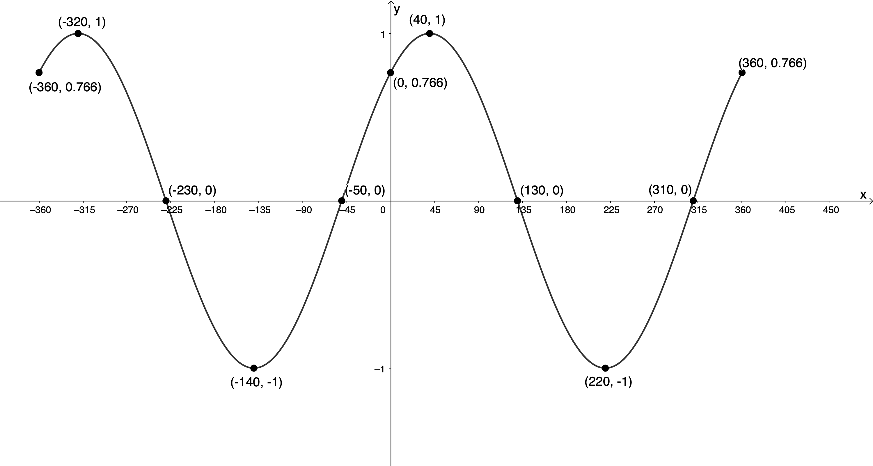
- [latex]\scriptsize h(x)=\cos (x-{{40}^\circ})[/latex] for [latex]\scriptsize -{{360}^\circ}\le x\le {{360}^\circ}[/latex]
[latex]\scriptsize p=-{{40}^\circ}[/latex]. Therefore, the graph will be shifted [latex]\scriptsize {{40}^\circ}[/latex] to the right.[latex]\scriptsize \cos x[/latex] [latex]\scriptsize ({{0}^\circ},1)[/latex] [latex]\scriptsize ({{90}^\circ},0)[/latex] [latex]\scriptsize ({{180}^\circ},-1)[/latex] [latex]\scriptsize ({{270}^\circ},0)[/latex] [latex]\scriptsize ({{360}^\circ},1)[/latex] [latex]\scriptsize \cos (x-{{40}^\circ})[/latex] [latex]\scriptsize ({{40}^\circ},1)[/latex] [latex]\scriptsize ({{130}^\circ},0)[/latex] [latex]\scriptsize ({{220}^\circ},-1)[/latex] [latex]\scriptsize ({{310}^\circ},0)[/latex] [latex]\scriptsize ({{400}^\circ},1)[/latex] .
y-intercept (let [latex]\scriptsize x=0[/latex]):
[latex]\scriptsize \begin{align*}h(0) & =\cos ({{0}^\circ}-{{40}^\circ})\\\therefore h(0) & =0.766\end{align*}[/latex]
.
Because the period of the function is [latex]\scriptsize {{360}^\circ}[/latex] we know that the function values at [latex]\scriptsize -{{360}^\circ}[/latex] and [latex]\scriptsize {{360}^\circ}[/latex] will also be [latex]\scriptsize 0.766[/latex].
.
Exercise 10.2
- [latex]\scriptsize y=-2\cos (x+{{30}^\circ})[/latex] for [latex]\scriptsize -{{360}^\circ}\le x\le {{360}^\circ}[/latex]
[latex]\scriptsize a=-2[/latex]. Therefore, the amplitude will be [latex]\scriptsize 2[/latex] and the graph will be reflected about the x-axis.
[latex]\scriptsize p={{30}^\circ}[/latex]. Therefore, the graph will be shifted [latex]\scriptsize {{30}^\circ}[/latex] to the left.[latex]\scriptsize \cos x[/latex] [latex]\scriptsize ({{0}^\circ},1)[/latex] [latex]\scriptsize ({{90}^\circ},0)[/latex] [latex]\scriptsize ({{180}^\circ},-1)[/latex] [latex]\scriptsize ({{270}^\circ},0)[/latex] [latex]\scriptsize ({{360}^\circ},1)[/latex] [latex]\scriptsize -2\cos (x+{{30}^\circ})[/latex] [latex]\scriptsize (-{{30}^\circ},-2)[/latex] [latex]\scriptsize ({{60}^\circ},0)[/latex] [latex]\scriptsize ({{150}^\circ},2)[/latex] [latex]\scriptsize ({{240}^\circ},0)[/latex] [latex]\scriptsize ({{330}^\circ},-2)[/latex] .
y-intercept (let [latex]\scriptsize x=0[/latex]):
[latex]\scriptsize \begin{align*}y & =-2\cos ({{0}^\circ}+{{30}^\circ})\\\therefore y & =-2\times \displaystyle \frac{{\sqrt{3}}}{2}\\=-\sqrt{3}=-1.732\end{align*}[/latex]
.
Because the period of the function is [latex]\scriptsize {{360}^\circ}[/latex] we know that the function values at [latex]\scriptsize -{{360}^\circ}[/latex] and [latex]\scriptsize {{360}^\circ}[/latex] will also be [latex]\scriptsize -1.732[/latex].
.
.
y-intercept: [latex]\scriptsize ({{0}^\circ},-1.732)[/latex]
x-intercepts: [latex]\scriptsize (-{{300}^\circ},0)[/latex], [latex]\scriptsize (-{{120}^\circ},0)[/latex], [latex]\scriptsize ({{60}^\circ},0)[/latex], [latex]\scriptsize ({{240}^\circ},0)[/latex]
Domain: [latex]\scriptsize \{x|x\in \mathbb{R},-{{360}^\circ}\le x\le {{360}^\circ}\}\text{ }[/latex]
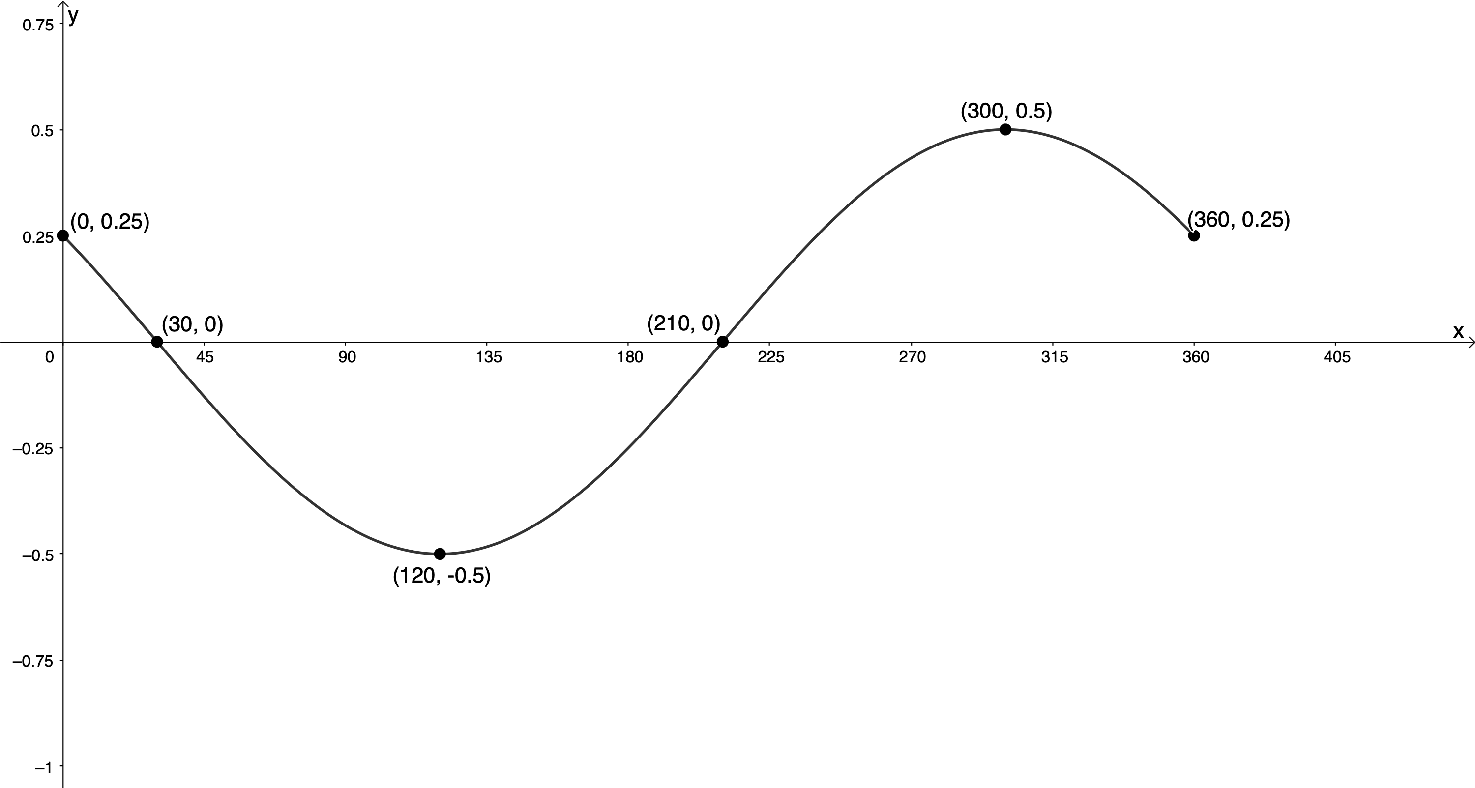
Range: [latex]\scriptsize \{y|y\in \mathbb{R},-2\le y\le 2\}\text{ }[/latex] - [latex]\scriptsize 2y=\cos (x+{{60}^\circ})[/latex] for [latex]\scriptsize {{0}^\circ}\le x\le {{360}^\circ}[/latex]
[latex]\scriptsize \begin{align*}2y & =\cos (x+{{60}^\circ})\\\therefore y & =\displaystyle \frac{1}{2}\cos (x+{{60}^\circ})\end{align*}[/latex]
[latex]\scriptsize a=\displaystyle \frac{1}{2}[/latex]. Therefore, the amplitude will be [latex]\scriptsize \displaystyle \frac{1}{2}[/latex].
[latex]\scriptsize p={{60}^\circ}[/latex]. Therefore, the graph will be shifted [latex]\scriptsize {{60}^\circ}[/latex] to the left.[latex]\scriptsize \cos x[/latex] [latex]\scriptsize ({{0}^\circ},1)[/latex] [latex]\scriptsize ({{90}^\circ},0)[/latex] [latex]\scriptsize ({{180}^\circ},-1)[/latex] [latex]\scriptsize ({{270}^\circ},0)[/latex] [latex]\scriptsize ({{360}^\circ},1)[/latex] [latex]\scriptsize \displaystyle \frac{1}{2}\cos (x+{{60}^\circ})[/latex] [latex]\scriptsize (-{{60}^\circ},\displaystyle \frac{1}{2})[/latex] [latex]\scriptsize ({{30}^\circ},0)[/latex] [latex]\scriptsize ({{120}^\circ},-\displaystyle \frac{1}{2})[/latex] [latex]\scriptsize ({{210}^\circ},0)[/latex] [latex]\scriptsize ({{300}^\circ},\displaystyle \frac{1}{2})[/latex] .
y-intercept (let [latex]\scriptsize x=0[/latex]):
[latex]\scriptsize \begin{align*}y & =\displaystyle \frac{1}{2}\cos ({{0}^\circ}+{{60}^\circ})\\\therefore y & =\displaystyle \frac{1}{2}\times \displaystyle \frac{1}{2}=\displaystyle \frac{1}{4}\end{align*}[/latex]
.
Because the period of the function is [latex]\scriptsize {{360}^\circ}[/latex] we know that the function value at [latex]\scriptsize {{360}^\circ}[/latex] will also be [latex]\scriptsize \displaystyle \frac{1}{4}[/latex].
.
.
y-intercept: [latex]\scriptsize ({{0}^\circ},0.25)[/latex] or [latex]\scriptsize ({{0}^\circ},\displaystyle \frac{1}{4})[/latex]
x-intercepts: [latex]\scriptsize ({{30}^\circ},0)[/latex], [latex]\scriptsize ({{210}^\circ},0)[/latex]
Domain: [latex]\scriptsize \{x|x\in \mathbb{R},{{0}^\circ}\le x\le {{360}^\circ}\}\text{ }[/latex]
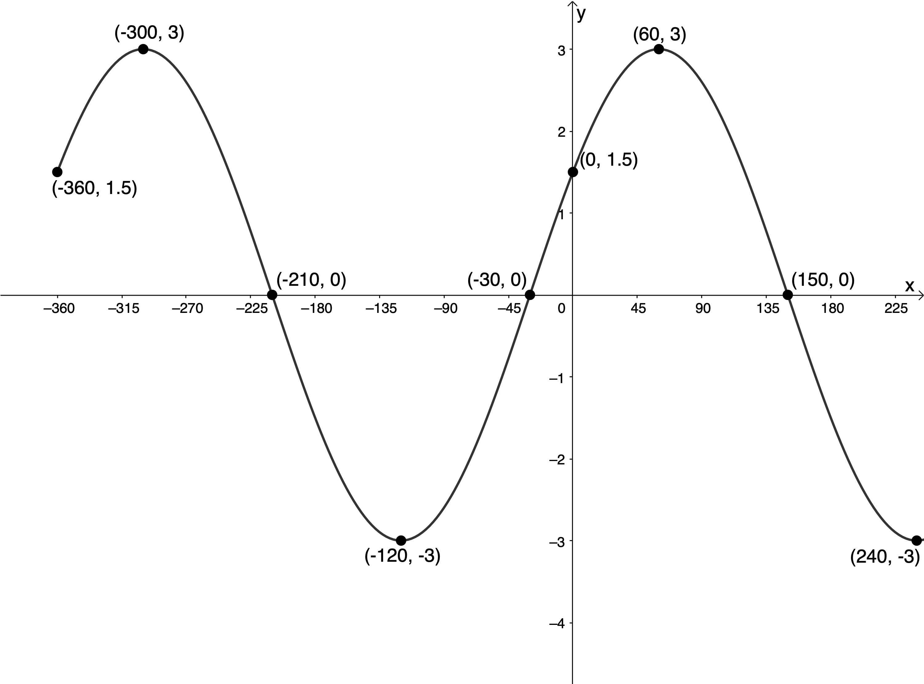
Range: [latex]\scriptsize \{y|y\in \mathbb{R},-\displaystyle \frac{1}{2}\le y\le \displaystyle \frac{1}{2}\}\text{ }[/latex] - [latex]\scriptsize \displaystyle \frac{1}{3}y=\cos ({{60}^\circ}-x)[/latex] for [latex]\scriptsize -{{360}^\circ}\le x\le {{360}^\circ}[/latex]
[latex]\scriptsize \begin{align*}\displaystyle \frac{1}{3}y & =\cos ({{60}^\circ}-x)\\\therefore y & =3\cos ({{60}^\circ}-x)\\&=3\cos (-x+{{60}^\circ})\\&=3\cos \left( {-\left( {x-{{{60}}^\circ}} \right)} \right)\\&=3\cos (x-{{60}^\circ})\end{align*}[/latex]
[latex]\scriptsize a=3[/latex]. Therefore, the amplitude will be [latex]\scriptsize 3[/latex].
[latex]\scriptsize p=-{{60}^\circ}[/latex]. Therefore, the graph will be shifted [latex]\scriptsize {{60}^\circ}[/latex] to the right.[latex]\scriptsize \cos x[/latex] [latex]\scriptsize ({{0}^\circ},1)[/latex] [latex]\scriptsize ({{90}^\circ},0)[/latex] [latex]\scriptsize ({{180}^\circ},-1)[/latex] [latex]\scriptsize ({{270}^\circ},0)[/latex] [latex]\scriptsize ({{360}^\circ},1)[/latex] [latex]\scriptsize 3\cos (x-{{60}^\circ})[/latex] [latex]\scriptsize ({{60}^\circ},3)[/latex] [latex]\scriptsize ({{150}^\circ},0)[/latex] [latex]\scriptsize ({{240}^\circ},-3)[/latex] [latex]\scriptsize ({{330}^\circ},0)[/latex] [latex]\scriptsize ({{420}^\circ},3)[/latex] .
y-intercept (let [latex]\scriptsize x=0[/latex]):
[latex]\scriptsize \begin{align*}y & =3\cos ({{0}^\circ}-{{60}^\circ})\\\therefore y & =-3\times \displaystyle \frac{1}{2}\\=\displaystyle \frac{3}{2}=1.5\end{align*}[/latex]
.
Because the period of the function is [latex]\scriptsize {{360}^\circ}[/latex] we know that the function values at [latex]\scriptsize -{{360}^\circ}[/latex] and [latex]\scriptsize {{360}^\circ}[/latex] will also be [latex]\scriptsize 1.5[/latex].
.
.
y-intercept: [latex]\scriptsize ({{0}^\circ},1.5)[/latex] or [latex]\scriptsize ({{0}^\circ},\displaystyle \frac{3}{2})[/latex]
x-intercepts: [latex]\scriptsize (-{{210}^\circ},0)[/latex], [latex]\scriptsize (-{{30}^\circ},0)[/latex], [latex]\scriptsize ({{150}^\circ},0)[/latex], [latex]\scriptsize ({{330}^\circ},0)[/latex]
Domain: [latex]\scriptsize \{x|x\in \mathbb{R},-{{360}^\circ}\le x\le {{360}^\circ}\}[/latex]
Range: [latex]\scriptsize \{y|y\in \mathbb{R},-3\le y\le 3\}[/latex]
Exercise 10.3
- Amplitude is [latex]\scriptsize 0.5=\displaystyle \frac{1}{2}[/latex]
The maximum turning point has been transformed to [latex]\scriptsize ({{45}^\circ},-\displaystyle \frac{1}{2})[/latex]. The graph has been shifted [latex]\scriptsize {{45}^\circ}[/latex] to the right and reflected about the x-axis. Therefore, [latex]\scriptsize a=-\displaystyle \frac{1}{2}[/latex] and [latex]\scriptsize p=-{{45}^\circ}[/latex].
[latex]\scriptsize y=-\displaystyle \frac{1}{2}\cos (x-{{45}^\circ})[/latex] - Domain: [latex]\scriptsize \{x|x\in \mathbb{R},\text{ }{{0}^\circ}\le x\le {{360}^\circ}\}[/latex]
Range: [latex]\scriptsize \{y|y\in \mathbb{R},\text{ }-\displaystyle \frac{1}{2}\le y\le \displaystyle \frac{1}{2}\}[/latex]
Unit 10: Assessment
- .
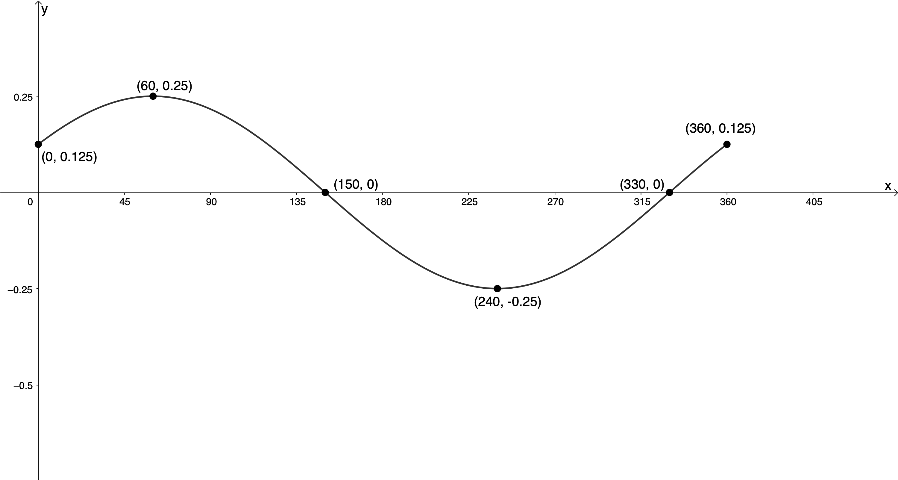
- [latex]\scriptsize 4y=\cos \left( {x-{{{60}}^\circ}} \right)[/latex] for [latex]\scriptsize {{0}^\circ}\le x\le {{360}^\circ}[/latex]
[latex]\scriptsize \begin{align*}4y & =\cos (x-{{60}^\circ})\\\therefore y & =\displaystyle \frac{1}{4}\cos (x-{{60}^\circ})\end{align*}[/latex]
[latex]\scriptsize a=\displaystyle \frac{1}{4}[/latex]. Therefore, the amplitude will be [latex]\scriptsize \displaystyle \frac{1}{4}[/latex].
[latex]\scriptsize p=-{{60}^\circ}[/latex]. Therefore, the graph will be shifted [latex]\scriptsize {{60}^\circ}[/latex] to the right.[latex]\scriptsize \cos x[/latex] [latex]\scriptsize ({{0}^\circ},1)[/latex] [latex]\scriptsize ({{90}^\circ},0)[/latex] [latex]\scriptsize ({{180}^\circ},-1)[/latex] [latex]\scriptsize ({{270}^\circ},0)[/latex] [latex]\scriptsize ({{360}^\circ},1)[/latex] [latex]\scriptsize \displaystyle \frac{1}{4}\cos (x-{{60}^\circ})[/latex] [latex]\scriptsize ({{60}^\circ},\displaystyle \frac{1}{4})[/latex] [latex]\scriptsize ({{150}^\circ},0)[/latex] [latex]\scriptsize ({{240}^\circ},-\displaystyle \frac{1}{4})[/latex] [latex]\scriptsize ({{330}^\circ},0)[/latex] [latex]\scriptsize ({{420}^\circ},\displaystyle \frac{1}{4})[/latex] .
y-intercept (let [latex]\scriptsize x=0[/latex]):
[latex]\scriptsize \begin{align*}y & =\displaystyle \frac{1}{4}\cos (0-{{60}^\circ})\\\therefore y & =\displaystyle \frac{1}{4}\times \displaystyle \frac{1}{2}=\displaystyle \frac{1}{8}=0.125\end{align*}[/latex]
.
Because the period of the function is [latex]\scriptsize {{360}^\circ}[/latex] we know that the function value at [latex]\scriptsize {{360}^\circ}[/latex] will also be [latex]\scriptsize 0.125[/latex].
.
- [latex]\scriptsize g(x)=-4\cos ({{45}^\circ}-x)[/latex] for [latex]\scriptsize -{{360}^\circ}\le x\le {{360}^\circ}[/latex]
[latex]\scriptsize \begin{align*}g(x) & =-4\cos ({{45}^\circ}-x)\\&=-4\cos (-x+{{45}^\circ})\\&=-4\cos \left( {-\left( {x-{{{45}}^\circ}} \right)} \right)\\&=-4\cos (x-{{45}^\circ})\end{align*}[/latex]
[latex]\scriptsize a=-4[/latex]. Therefore, the amplitude will be [latex]\scriptsize 4[/latex] and the graph will be reflected about the x-axis.
[latex]\scriptsize \displaystyle p=-{{45}^\circ}[/latex]. Therefore, the graph will be shifted [latex]\scriptsize {{45}^\circ}[/latex] to the right.[latex]\scriptsize \cos x[/latex] [latex]\scriptsize ({{0}^\circ},1)[/latex] [latex]\scriptsize ({{90}^\circ},0)[/latex] [latex]\scriptsize ({{180}^\circ},-1)[/latex] [latex]\scriptsize ({{270}^\circ},0)[/latex] [latex]\scriptsize ({{360}^\circ},1)[/latex] [latex]\scriptsize -4\cos (x-{{45}^\circ})[/latex] [latex]\scriptsize ({{45}^\circ},-4)[/latex] [latex]\scriptsize ({{135}^\circ},0)[/latex] [latex]\scriptsize ({{225}^\circ},4)[/latex] [latex]\scriptsize ({{315}^\circ},0)[/latex] [latex]\scriptsize ({{405}^\circ},-4)[/latex] .
y-intercept (let [latex]\scriptsize x=0[/latex]):
[latex]\scriptsize \begin{align*}g(0)&=-4\cos (0-{{45}^\circ})\\\therefore y & =-4\times \displaystyle \frac{1}{{\sqrt{2}}}=-2.828\end{align*}[/latex]
.
Because the period of the function is [latex]\scriptsize {{360}^\circ}[/latex] we know that the function values at [latex]\scriptsize -{{360}^\circ}[/latex] and [latex]\scriptsize {{360}^\circ}[/latex] will also be [latex]\scriptsize -2.828[/latex].
.

- [latex]\scriptsize 4y=\cos \left( {x-{{{60}}^\circ}} \right)[/latex] for [latex]\scriptsize {{0}^\circ}\le x\le {{360}^\circ}[/latex]
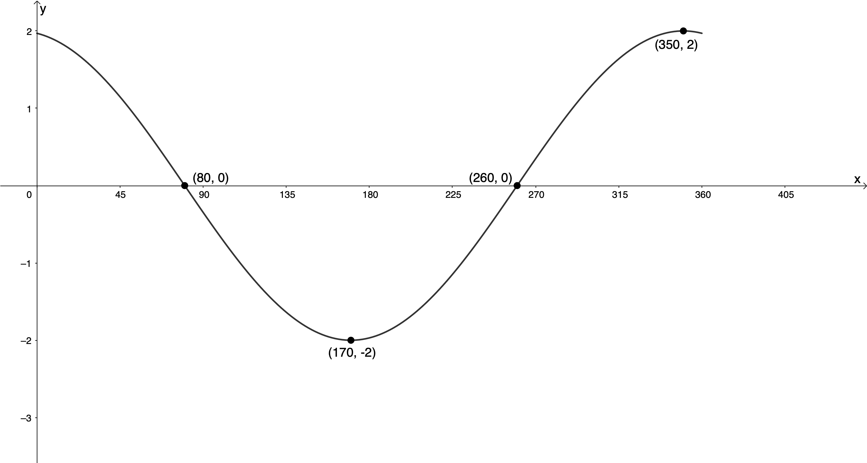
- The function is of the form [latex]\scriptsize y=a\cos (x+p)[/latex]. The amplitude is [latex]\scriptsize 2[/latex]. The minimum turning point [latex]\scriptsize ({{180}^\circ},-1)[/latex] has been transformed to [latex]\scriptsize ({{170}^\circ},-2)[/latex]. The graph has been shifted [latex]\scriptsize {{10}^\circ}[/latex] to the left. Therefore, [latex]\scriptsize a=2[/latex] and [latex]\scriptsize p={{10}^\circ}[/latex]. The function is [latex]\scriptsize y=2\cos (x+{{10}^\circ})[/latex].
- .
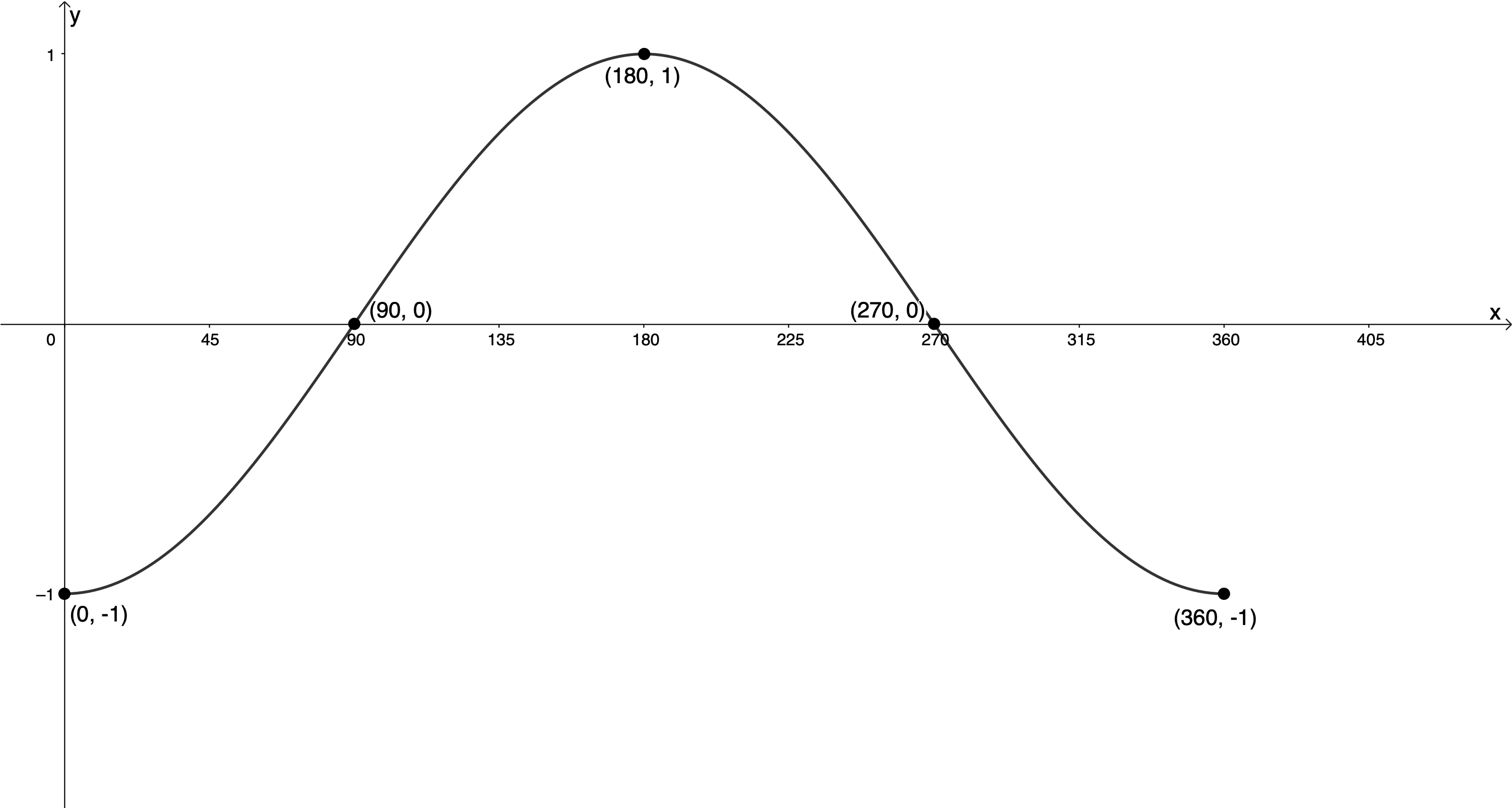
- [latex]\scriptsize y=a\cos x[/latex] shows no horizontal shift. The maximum turning point that was at [latex]\scriptsize ({{0}^\circ},1)[/latex] is now at [latex]\scriptsize ({{0}^\circ},-1)[/latex]. Therefore, the amplitude is [latex]\scriptsize 1[/latex] but the graph has been reflected about the x-axis. Therefore, [latex]\scriptsize y=-\cos x[/latex].
- [latex]\scriptsize y=\cos (x+p)[/latex] means that the function has undergone a horizontal shift. The maximum turning point that was at [latex]\scriptsize ({{0}^\circ},1)[/latex] is now at [latex]\scriptsize ({{180}^\circ},1)[/latex]. In other words, the graph has been shifted [latex]\scriptsize {{180}^\circ}[/latex] to the right. Therefore [latex]\scriptsize y=\cos (x-{{180}^\circ})[/latex].
Alternatively, we can say that the maximum turning point that was at [latex]\scriptsize ({{360}^\circ},1)[/latex] is now at [latex]\scriptsize ({{180}^\circ},1)[/latex] and that the graph has been shifted [latex]\scriptsize {{180}^\circ}[/latex] to the left and [latex]\scriptsize y=\cos (x+{{180}^\circ})[/latex] - [latex]\scriptsize y=\sin (x+p)[/latex] means that the function has undergone a horizontal shift. The maximum turning point that was at [latex]\scriptsize ({{90}^\circ},1)[/latex] is now at [latex]\scriptsize ({{180}^\circ},1)[/latex]. Therefore, the graph has been shifted [latex]\scriptsize {{90}^\circ}[/latex] to the right and [latex]\scriptsize y=\sin (x-{{90}^\circ})[/latex]
Media Attributions
- takenote © DHET is licensed under a CC BY (Attribution) license
- example10.1 © Geogebra is licensed under a CC BY-SA (Attribution ShareAlike) license
- example10.2 © Geogebra is licensed under a CC BY-SA (Attribution ShareAlike) license
- example10.3 © Geogebra is licensed under a CC BY-SA (Attribution ShareAlike) license
- example10.4 © Geogebra is licensed under a CC BY-SA (Attribution ShareAlike) license
- example10.5 © Geogebra is licensed under a CC BY-SA (Attribution ShareAlike) license
- exercise10.3 © Geogebra is licensed under a CC BY-SA (Attribution ShareAlike) license
- figure7 © Geogebra is licensed under a CC BY-SA (Attribution ShareAlike) license
- figure8 © Geogebra is licensed under a CC BY-SA (Attribution ShareAlike) license
- figure9 © Geogebra is licensed under a CC BY-SA (Attribution ShareAlike) license
- figure10 © Geogebra is licensed under a CC BY-SA (Attribution ShareAlike) license
- figure11 © DHET is licensed under a CC BY-SA (Attribution ShareAlike) license
- assessmentQ2 © Geogebra is licensed under a CC BY-SA (Attribution ShareAlike) license
- assessmentQ3 © Geogebra is licensed under a CC BY-SA (Attribution ShareAlike) license
- exercise10.1A1 © Geogebra is licensed under a CC BY-SA (Attribution ShareAlike) license
- exercise10.1A2 © Geogebra is licensed under a CC BY-SA (Attribution ShareAlike) license
- exercise10.1A3 © Geogebra is licensed under a CC BY-SA (Attribution ShareAlike) license
- exercise10.2A1 © Geogebra is licensed under a CC BY-SA (Attribution ShareAlike) license
- exercise10.2A2 © Geogebra is licensed under a CC BY-SA (Attribution ShareAlike) license
- exercise10.2A3 © Geogebra is licensed under a CC BY-SA (Attribution ShareAlike) license
- assessmentA1a © Geogebra is licensed under a CC BY-SA (Attribution ShareAlike) license
- assessmentA1b © Geogebra is licensed under a CC BY-SA (Attribution ShareAlike) license
