Data handling: Calculate, represent and interpret measures of central tendency and dispersion in univariate numerical ungrouped data
Unit 1: Revise measures of central tendency and dispersion for ungrouped data
Natashia Bearam-Edmunds
Unit outcomes
By the end of this unit you will be able to:
- Find the mean for ungrouped data.
- Find the median for ungrouped data.
- Find the mode for ungrouped data.
- Find the range and interquartile range.
What you should know
Before you start this unit, make sure you can:
- Calculate central tendencies and dispersion of data and represent data effectively. Revise the following level 2, topic 4 units on data handling:
- Subject outcome 4.1, unit 1: data collecting.
- Subject outcome 4.1, unit 2: measures of central tendency of ungrouped data.
- Subject outcome 4.1, unit 3: measures of dispersion of ungrouped data.
- Subject outcome 4.2, unit 1: data representation.
- Subject outcome 4.2, unit 2: bar graphs and histograms.
- Subject outcome 4.2, unit 3: frequency polygon and line graphs.
Introduction
You will come across many formulas to calculate . The purpose of statistics is not to perform numerous calculations using formulas, but to gain an understanding of your data. The calculations are often done using a calculator or a computer but basic calculations can be done by hand too. The understanding must come from you. If you can thoroughly understand the basics of statistics, you can be more confident in the decisions you make in life.
In this unit, we revise how to calculate statistics that give us information about the central values and spread of data.
Let’s revise the terms that you should know by doing Activity 1.1.
Activity 1.1: Define the key terms used in data handling
Time required: 10 minutes
What you need:
- a pen and paper
What to do:
Read the following and answer the questions:
We want to study the average amount of money first year learners spend at ABC College on supplies that do not include books. We randomly surveyed 100 first year learners at the college. Three of those learners spent [latex]\scriptsize \text{R }1000,\text{ R }850[/latex] and [latex]\scriptsize \text{R }500[/latex].
- What is the population in the study?
- What is the sample in the study?
- State the parameter.
- State the statistic.
- What are the possible variables being studied?
- Write another word for ‘average’.
- What are the data values?
What did you find?
- A population is a collection of persons, things or objects under study. The population in this study is all first year learners attending ABC College.
- To study the population, we select a sample. The sample could be all enrolled in a beginning statistics course at ABC College (although this sample may not represent the entire population). In this study [latex]\scriptsize 100[/latex] learners make up the sample. The bigger the sample size is the more closely it will represent the population.
- A parameter is a number used to represent a population characteristic and cannot be easily found hence it is estimated by a statistic. The parameter in this study is the average amount of money spent (excluding books) by all first year learners at ABC College.
- The statistic is the average amount of money spent (excluding books) by first year college learners in the sample.
- The variable could be the amount of money spent (excluding books) by one first year learner. For example, let [latex]\scriptsize \displaystyle X=[/latex] the amount of money spent (excluding books) by one first year learner at the college.
- The ‘average’ is also called the ‘mean’; a number that describes the central tendency of data.
- Data are the actual values of the variable. The data are the rand amounts spent by the first year learners, or example [latex]\scriptsize \text{R }1000,\text{ R }850[/latex] and [latex]\scriptsize \text{R }500[/latex].
Data are either qualitative or quantitative. Qualitative data describe features. Car colour, race and blood type are examples of qualitative data.
Quantitative data are numbers and the result of counting or measuring. Weight, pulse rate and number of people are examples of quantitative data. Quantitative data is further divided into:
- discrete data – this data takes on only certain numerical values and can be counted, for example the number of days.
- continuous data – this data can be measured and include fractions, decimals or irrational numbers, for example time.
Data in its raw form is called ungrouped data. Once the data has been organised using frequencies we call this grouped data. We use different methods to calculate measures of central tendency for ungrouped and grouped data
Measures of central tendency for ungrouped data
We can summarise data by calculating measures of central tendency and dispersion. In this unit we will focus on the measures of central tendency, which are the mean, median and mode.
The mean
The mean (average) and the median are the two measures of central tendency that are used most widely. Of the three measures of central tendency, the mean is most heavily influenced by any outliers or skewness in data. When there are outliers in the data, the median is often the preferred measure of central tendency because the median is more resistant to outliers than the mean.
To calculate the mean we add all the data values and divide by the total number of values. For example, to calculate your average mark for three maths tests you would add the three marks together and divide by three. We can write this as a formula as shown below.
Mean for ungrouped data:
[latex]\scriptsize \bar{x}=\displaystyle \frac{{\sum\limits_{{i=1}}^{n}{{{{x}_{i}}}}}}{n}[/latex]
[latex]\scriptsize \displaystyle \bar{x}[/latex] called ‘[latex]\scriptsize \displaystyle ~x[/latex]bar’ indicates the mean
[latex]\scriptsize n[/latex] is the total number of data values
[latex]\scriptsize \Sigma[/latex] is the sum of the data
[latex]\scriptsize \displaystyle {{x}_{i}}[/latex] are the data values
Let’s look at an example to better understand these measures of central tendency.
Example 1.1
Exam scores for [latex]\scriptsize 11[/latex] learners are as follows:
[latex]\scriptsize \displaystyle 50;\text{ }58;\text{ 6}9;\text{ 42};\text{ }63;\text{ 72};\text{ 5}2;\text{ 80};\text{ 65};\text{ }72;\text{ 91}[/latex]
- Calculate the mean mark.
- How many learners received better than average marks?
- Adam got [latex]\scriptsize 63\%[/latex]he believes that his mark is better than the average because it is greater than [latex]\scriptsize 50\%[/latex]. Is he correct? Explain.
Solution
- Using the formula for the mean, we find the sum of the exam scores and then divide by the number of values.
[latex]\scriptsize \displaystyle \begin{align*}\bar{x}&=\displaystyle \frac{{\sum\limits_{{i=1}}^{n}{{{{x}_{i}}}}}}{n}\\&=\displaystyle \frac{{50+58+\text{6}9+\text{42+}63+\text{72+5}2+\text{80+65+}72+\text{91}}}{{11}}\\&=\displaystyle \frac{{714}}{{11}}\\&=64.9\%\end{align*}[/latex]
.
How to use the Casio fx-82ZA Plus to find the mean for ungrouped data:
Step 1: Start with the calculator turned off. Turn the calculator on then set the calculator to statistics (MODE 2) and press [latex]\scriptsize 1[/latex] for [latex]\scriptsize 1[/latex] variable statistics. If the calculator has a frequency column showing turn the frequency off by pressing SHIFT, MODE (SET UP), REPLAY down, [latex]\scriptsize 3[/latex] for statistics then [latex]\scriptsize 2[/latex] for ‘off’. For ungrouped data make sure frequency is turned off.Step 2: Enter the data. Press [latex]\scriptsize 50[/latex] then [latex]\scriptsize =[/latex] [latex]\scriptsize 58=[/latex] [latex]\scriptsize 69=[/latex] and so on until you enter [latex]\scriptsize 91=[/latex]. If you make a mistake, don‛t worry! Simply scroll up to the wrong data value and type the correct value over it.
Step 3: After you have finished entering the scores, press AC to indicate the completion of the data entering stage. Don‛t panic when the scores disappear! The data entering screen will disappear but can be brought back if needed.
Step 4: To bring up the value for the mean press SHIFT [latex]\scriptsize 1[/latex] then [latex]\scriptsize 4:\text{VAR}[/latex] next press [latex]\scriptsize 2:\overline{x}=[/latex] and the value of [latex]\scriptsize 64.9[/latex] is displayed.
- Five learners scored more than [latex]\scriptsize 64.9\%[/latex] on the test.
- No he is not correct. The average test mark is [latex]\scriptsize 64.9\%[/latex] not [latex]\scriptsize 50\%[/latex] and with a mark of [latex]\scriptsize 63\%[/latex] he scored below the average.
Exercise 1.1
- AIDS data indicating the number of months a patient with AIDS lives after taking a new antibody drug are as follows:
[latex]\scriptsize \displaystyle \begin{align*}&\text{3; 4; 8; 8; 10; 11; 12; 13; 14; 15; 15; 16; 16; 17; 17; 18; 21; 22; 22; 24; 24; 25; 26; 26; 27; 27; }\\ &\text{29; 29; 31; 32; 33; 33; 34; 34; 35; 37; 40; 44; 44; 47}\end{align*}[/latex]Calculate the mean and explain what the statistic you have found represents.
- Statistics can be used to compare anything, in this case authors. The following shows a simple random sample that compares the letter counts for the first words used by three authors in ten articles they wrote.
Terry: [latex]\scriptsize \displaystyle \text{7; 9; 3; 3; 3; 4; 1; 3; 2; 2}[/latex]
Davis: 3; 3; 3; 4; 1; 4; 3; 2; 3; 1
Maris: 2; 3; 4; 4; 4; 6; 6; 6; 8; 3Calculate the mean letter count for each author.
The full solutions are at the end of the unit.
The median
The median is the middle value of an ordered data set. To find the median, we first sort the data in increasing order and then pick out the value in the middle of the sorted list. The median is the best measure of the centre when a data set contains outliers or extreme values.
Example 1.2
We will once again use the exam scores for [latex]\scriptsize 11[/latex] learners, which are as follows:
[latex]\scriptsize \displaystyle 50;\text{ }58;\text{ 6}9;\text{ 42};\text{ }63;\text{ 72};\text{ 5}2;\text{ 80};\text{ 65};\text{ }72;\text{ 91}[/latex]
Find the median and state how many learners scored marks below the median value and how many scored marks above the median.
Solution
To find the median, we must first order the data.
[latex]\scriptsize \displaystyle 42;\text{ }50;\text{ 52; }58;\text{ 63; 65; 6}9;\text{ 72};\text{ 72; 80};\text{ 91}[/latex]
You can quickly find the location of the median by using: [latex]\scriptsize \displaystyle \frac{{n+1}}{2}[/latex]
If [latex]\scriptsize n[/latex] is an odd number, the median is the middle value of the ordered data (ordered smallest to largest). If [latex]\scriptsize n[/latex] is an even number, the median is equal to the two middle values added together and divided by two after the data has been ordered.
Since there are an odd number of values the median will be the middle value after ordering the data.
Position of the median is [latex]\scriptsize \displaystyle \frac{{11+1}}{2}=6[/latex]
[latex]\scriptsize \displaystyle 42;\text{ }50;\text{ 52; }58;\text{ 63; }\underline{{\text{65}}}\text{; 6}9;\text{ 72};\text{ 72; 80};\text{ 91}[/latex]
Count six places from the beginning of the ordered list and you will find that the sixth value is [latex]\scriptsize 65[/latex] therefore the median mark is [latex]\scriptsize 65[/latex].
The median divides the data into two equal parts so [latex]\scriptsize 50\%[/latex] of data values lie below the median and [latex]\scriptsize 50\%[/latex] of values lie above it. There are five marks below [latex]\scriptsize 65[/latex] and five marks above [latex]\scriptsize 65[/latex].
Exercise 1.2
- Looking again at the same AIDS data which indicate the number of months a patient with AIDS lives after taking a new antibody drug. The data are as follows:
[latex]\scriptsize \displaystyle \begin{align*}&\text{3; 4; 8; 8; 10; 11; 12; 13; 14; 15; 15; 16; 16; 17; 17; 18; 21; 22; 22; 24; 24; 25; 26; 26; 27; 27; }\\ &\text{29; 29; 31; 32; 33; 33; 34; 34; 35; 37; 40; 44; 44; 47}\end{align*}[/latex]
Calculate the median. - Suppose that in a small town of [latex]\scriptsize \displaystyle 50[/latex] people, one person earns [latex]\scriptsize \displaystyle \text{R}5\text{ }000\text{ }000[/latex] per year and the other [latex]\scriptsize \displaystyle 49[/latex] each earn [latex]\scriptsize \displaystyle \text{R}30\text{ }000[/latex] a year. Which is the better measure of the ‘centre’; the mean or the median? Explain your reasoning.
- In a sample of [latex]\scriptsize \displaystyle 60[/latex] houses, one house is worth [latex]\scriptsize \displaystyle \text{R}2\text{ }500\text{ }000[/latex]. Half of the rest are worth [latex]\scriptsize \displaystyle \text{R}280\text{ }000[/latex], and all the others are worth [latex]\scriptsize \displaystyle \text{R350 }000[/latex]. Without doing any calculations, which is the better measure of the “centre” house value; the mean or the median?
The full solutions are at the end of the unit.
The mode
The mode is the most frequent value. There can be more than one mode in a data set. A data set with two modes is called bimodal.
Example 1.3
The number of books checked out from the library by [latex]\scriptsize \displaystyle 25[/latex] learners are as follows:
[latex]\scriptsize \displaystyle \text{0; 0; 0; 1; 2; 3; 3; 4; 4; 5; 5; 7; 7; 7; 7; 8; 8; 8; 9; 10; 10; 11; 11; 12; 12}[/latex]
Find the mode.
Solution
It is easier to pick out the mode if the data are ordered. The mode is [latex]\scriptsize 7[/latex] as it is repeated the most often ([latex]\scriptsize 4[/latex] times).
Exercise 1.3
- Look at the following set of numbers:
[latex]\scriptsize \displaystyle 6;\text{ }7;\text{ }11;\text{ }10;\text{ }15;\text{ }13;\text{ }14;\text{ }8[/latex]- Notice in this data set there are an even number of values. What should you do first to find the average of these numbers?
- Write down the steps you would use to find the median.
- Find the mean of the data.
- Is it possible to calculate the mode of the data? Will it be a useful measure in this case?
- What word describes a distribution that has two modes?
The full solutions are at the end of the unit.
Note
To review measures of central tendency and the shape of distributions you can watch this video when you have an internet connection.
Measures of dispersion for ungrouped data
Measures of dispersion tell us how spread out a data set is. If a measure of dispersion is small, the data are clustered in a small region. If a measure of dispersion is large, the data are spread out over a large region. In this section we revise the measures of dispersion, the range and interquartile range.
The simplest measure of dispersion is the range. The range is the difference between the maximum and minimum values of the data set.
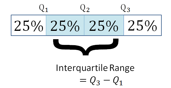
Quartiles divide data into four equal parts. The quartiles are computed in a similar way to the median. The median is halfway into the ordered data set and is also called the second quartile.
The first quartile [latex]\scriptsize ({{\text{Q}}_{1}})[/latex] is one quarter of the way into the ordered data set; whereas the third quartile [latex]\scriptsize \displaystyle ({{\text{Q}}_{3}})[/latex] is three quarters of the way into the ordered data set. The data must be ordered before you can calculate the quartiles.
The inter-quartile range is the difference between the first and third quartiles of the data set.
Activity 1.2: Calculate the range and interquartile range (IQR)
Time required: 25 minutes
What you need:
- a pen and paper
What to do:
Answer these questions and show all the necessary steps.
The data below gives the heights (in mm) of seedlings [latex]\scriptsize 4[/latex] weeks after germinating:
[latex]\scriptsize \displaystyle 47;\text{ }52;\text{ }56;\text{ }62;\text{ }71;\text{ }74;\text{ }78;\text{ }86;\text{ }89;\text{ }92;\text{ }93;\text{ }95[/latex]
- Calculate the median.
- Divide the data into an upper half and lower half.
- Find the median of the lower half of the data. What have you found?
- Find the median of the upper half of the data. What have you found?
- How many parts has the data been divided into?
- Find the difference between the values in 3 and 4 above. What have you found?
- Between what heights do [latex]\scriptsize 50\%[/latex] of the seedlings lie?
- Find the difference between the tallest and shortest seedling. What do we call this?
What did you find?
- The data is already arranged from lowest to highest and has [latex]\scriptsize \displaystyle 12[/latex] entries. To find the position of the median: [latex]\scriptsize \displaystyle \frac{{n+1}}{2}=\displaystyle \frac{{12+1}}{2}=6.5[/latex].
To find the median we must add the [latex]\scriptsize \displaystyle 6\text{th}[/latex] and [latex]\scriptsize \displaystyle 7\text{th}[/latex] data values and divide by [latex]\scriptsize 2[/latex]:
[latex]\scriptsize \text{M}=\displaystyle \frac{{74+78}}{2}=76\text{ mm}[/latex]
The median divides the data into an upper and lower half and is located between [latex]\scriptsize \displaystyle 74[/latex] and [latex]\scriptsize \displaystyle 78[/latex].
[latex]\scriptsize \displaystyle \begin{align*}\text{Lower half: }47;\text{ }52;\text{ }56;\text{ }62;\text{ }71;\text{ }74\\\text{Upper half: }78;\text{ }86;\text{ }89;\text{ }92;\text{ }93;\text{ }95\end{align*}[/latex] - We must find the median of the lower half of the data, which is called the first quartile and represented by [latex]\scriptsize {{\text{Q}}_{\text{1}}}[/latex]. The first quartile (also called the lower quartile) has [latex]\scriptsize \displaystyle 25\%[/latex] of data (scores) below it; it is the median of the lower [latex]\scriptsize \displaystyle 50\%[/latex] of the data. It is found between the [latex]\scriptsize \displaystyle 3\text{rd}[/latex] and [latex]\scriptsize \displaystyle ~4\text{th}[/latex] values.
[latex]\scriptsize \begin{align*}{{\text{Q}}_{\text{1}}}&=\text{ first }\!\!~\!\!\text{ quartile}\\&=\displaystyle \frac{{56+62}}{2}\\&=59\text{ mm}\end{align*}[/latex] - The median of the upper half of the data is called the upper or third quartile and is represented as [latex]\scriptsize {{\text{Q}}_{3}}[/latex]. The third quartile has [latex]\scriptsize \displaystyle 75\%[/latex] of the data (scores) below it. It will be located between the [latex]\scriptsize \displaystyle 9\text{th}[/latex] and [latex]\scriptsize \displaystyle 10\text{ th}[/latex]value of the original data set.
[latex]\scriptsize \begin{align*}{{\text{Q}}_{3}}&=\text{third }\!\!~\!\!\text{ quartile}\\&=\displaystyle \frac{{89+92}}{2}\\&=90.5\text{ mm}\end{align*}[/latex] - The data has been divided into four parts.
- We can use the first quartile and third quartile to compute the IQR.
[latex]\scriptsize \begin{align*}\text{IQR}&={{\text{Q}}_{3}}-{{\text{Q}}_{1}}\\&=90,5-59\\&=31.5\text{ mm}\end{align*}[/latex] - [latex]\scriptsize 50\%[/latex] of the seedlings are between [latex]\scriptsize 59\text{ mm}[/latex] and [latex]\scriptsize 90.5\text{ mm}[/latex] in height.
- [latex]\scriptsize \text{Tallest}-\text{shortest}=95-47=48\text{ mm}[/latex]
- The difference between the largest and smallest values in a data set is called the range.
An outlier is a data point that is significantly different from the other data points. The IQR can help to determine potential outliers.
A value is suspected to be a potential outlier if it is less than [latex]\scriptsize \displaystyle 1.5\times \text{IQR}[/latex] below the first quartile or more than [latex]\scriptsize \displaystyle 1.5\times \text{IQR}[/latex] above the third quartile. Potential outliers always require further investigation, for example, investigating the effect that it has on the data set as a whole.
Exercise 1.4
- For the following [latex]\scriptsize \displaystyle 13[/latex] house prices, calculate the IQR and determine if any prices are potential outliers.
[latex]\scriptsize \displaystyle \begin{align*}&389\text{ }950;\text{ }230\text{ }500;\text{ }158\text{ }000;\text{ }479\text{ }000;\text{ }639\text{ }000;\text{ }114\text{ }950;\text{ }5\text{ }500\text{ }000;\text{ }387\text{ }000;\text{ }\\&659\text{ }000;\text{ }529\text{ }000;\text{ }575\text{ }000;\text{ }488\text{ }800;\text{ }1\text{ }095\text{ }000\end{align*}[/latex] - The table below summarises two data sets of test scores for an evening statistics class and a daytime statistics class.
Min [latex]\scriptsize ({{\text{Q}}_{1}})[/latex] Median [latex]\scriptsize ({{\text{Q}}_{3}})[/latex] Maximum Day [latex]\scriptsize 32[/latex] [latex]\scriptsize 56[/latex] [latex]\scriptsize 74.5[/latex] [latex]\scriptsize 82.5[/latex] [latex]\scriptsize 99[/latex] Night [latex]\scriptsize 25.5[/latex] [latex]\scriptsize 78[/latex] [latex]\scriptsize 81[/latex] [latex]\scriptsize 89[/latex] [latex]\scriptsize 98[/latex] - Find the IQR for both classes. Compare and comment on the two IQRs.
- Are there outliers in either of the classes? Provide reasons for your answer.
The full solutions are at the end of the unit.
Summary
In this unit you have learnt the following:
- How to find the mean for ungrouped data by hand and by using a calculator.
- How to find the median and mode for ungrouped data.
- How to find the range and interquartile range for ungrouped data.
Unit 1: Assessment
Suggested time to complete: 30 minutes
- Sixty-five randomly selected car salespeople were asked the number of cars they generally sell in one week. Fourteen people answered that they generally sell three cars; nineteen generally sell four cars; twelve generally sell five cars; nine generally sell six cars; eleven generally sell seven cars.
- Calculate the sample mean.
- Find the median.
- Find the mode.
- Of the three measures, which tends to reflect skewing the most; the mean, the mode, or the median? Why?
- Sharpe School is applying for a grant that will be used to add fitness equipment to the school gym. The principal surveyed [latex]\scriptsize \displaystyle 15[/latex] anonymous learners to determine how many minutes a day the learners spend exercising. The results from the learners are shown: [latex]\scriptsize \displaystyle \begin{align*}&{0\text{ minutes; }40\text{ minutes; }60\text{ minutes; }30\text{ minutes; 60 minutes;}} \\&{10\text{ minutes; }45\text{ minutes; }30\text{ minutes; }300\text{ minutes; }90\text{ minutes;}} \\&{30\text{ minutes; }120\text{ minutes; }60\text{ minutes; }0\text{ minutes; }20\text{ minutes}} \end{align*}[/latex]
- Determine the following five values of the data:
minimum, first quartile, median, third quartile and maximum. - If you were the principal, would you be justified in purchasing new fitness equipment? Calculate the IQR and any potential outliers and note any pitfalls the principal should be aware of as part of your answer.
- Determine the following five values of the data:
The full solutions are at the end of the unit.
Unit 1: Solutions
Exercise 1.1
- .
[latex]\scriptsize \displaystyle \begin{align*}\bar{\text{x}}&=\displaystyle \frac{{\text{3+4+2(8)+10+11+}...\text{+44(2)+47}}}{{40}}\\&=\displaystyle \frac{{944}}{{40}}\\&=23.6\end{align*}[/latex]
On average a patient will live [latex]\scriptsize 23.6[/latex] months after taking the new antibody drug. - .
Terry’s mean:
[latex]\scriptsize \displaystyle \frac{{\text{7+9+4(3)+4+1+2(2)}}}{{10}}=3.7[/latex]
Davis’ mean:
[latex]\scriptsize \displaystyle \frac{{\text{5(3)+2(4)+2(1)+2}}}{{10}}=2.7[/latex]
Maris’ mean:
[latex]\scriptsize \displaystyle \frac{{\text{2+2(3)+3(4)+3(6)+8}}}{{10}}=4.6[/latex]
Exercise 1.2
- To find the median, M, first use the formula for the location. The location is: [latex]\scriptsize \displaystyle \frac{{n+1}}{2}=\displaystyle \frac{{41}}{2}=20.5[/latex]. Starting at the smallest value, the median is located between the [latex]\scriptsize \displaystyle 20\text{th}[/latex] and [latex]\scriptsize \displaystyle 21\text{st}[/latex] values (the two [latex]\scriptsize \displaystyle 24\text{s}[/latex]):
[latex]\scriptsize \displaystyle \begin{align*}&\text{3; 4; 8; 8; 10; 11; 12; 13; 14; 15; 15; 16; 16; 17; 17; 18; 21; 22; 22; }\underline{{\text{24; 24}}}\text{; 25; 26; 26; 27; 27; }\\&\text{29; 29; 31; 32; 33; 33; 34; 34; 35; 37; 40; 44; 44; 47}\end{align*}[/latex]
[latex]\scriptsize \displaystyle \begin{align*}\text{M}&=\displaystyle \frac{{24+24}}{2}\\&=24\end{align*}[/latex] - Calculate the mean then the median and compare.
[latex]\scriptsize \begin{align*}\bar{x}&=\displaystyle \frac{{5\text{ }000\text{ }000+49(30\text{ }000)}}{{50}}\\&=129\text{ }400\end{align*}[/latex]
The mean is [latex]\scriptsize \text{R}129\text{ 4}00[/latex]
.
[latex]\scriptsize \text{M}=30\text{ }000[/latex]. The median is [latex]\scriptsize \text{R}30\text{ }000[/latex] (since there are [latex]\scriptsize \displaystyle 49[/latex] people who earn [latex]\scriptsize \text{R}30\text{ }000[/latex] and one person who earns [latex]\scriptsize \text{R}5\text{ 00}0\text{ }000[/latex] and the median is in position [latex]\scriptsize \displaystyle 25.5[/latex]).
The median is a better measure of the centre of the data than the mean because [latex]\scriptsize \displaystyle 49[/latex] of the values are [latex]\scriptsize \text{R}30\text{ }000[/latex] and only one is [latex]\scriptsize \text{R}5\text{ 00}0\text{ }000[/latex]. The [latex]\scriptsize \text{R}5\text{ 00}0\text{ }000[/latex] is an outlier. The [latex]\scriptsize \text{R}30\text{ }000[/latex] gives us a better sense of the middle of the data. - The median will be a better indication of the middle of the data as most of the data values lie between [latex]\scriptsize \displaystyle \text{R}280\text{ }000[/latex] and [latex]\scriptsize \displaystyle \text{R35}0\text{ }000[/latex]. [latex]\scriptsize \displaystyle \text{R}2\text{ }500\text{ }000[/latex] is an outlier and will cause the mean value to be increased and give an incorrect indication of the centre of the data.
Exercise 1.3
- .
- Find the sum of the data values.
- Step 1: Order the data set from least to greatest.
Step 2: Find the position of the median using the formula [latex]\scriptsize \displaystyle \frac{{n+1}}{2}[/latex] .
Since there is an even number of items in the data set, the median is found by taking the mean (average) of the two middlemost numbers.Step 3: Write down the median.
- .
[latex]\scriptsize \begin{align*}\bar{x} &=\displaystyle \frac{{6+7+11+10+15+13+14+8}}{8}\\&=10.5\end{align*}[/latex] - There is no mode as no number occurs more than once. The mode will not be useful in this case, the mean and median are equal therefore the distribution would be symmetric.
- Bimodal.
Exercise 1.4
- Order the data from smallest to largest value.
[latex]\scriptsize \displaystyle \begin{align*}&114\text{ }950;\text{ }158\text{ }000;\text{ }230\text{ }500;\text{ }387\text{ }000;\text{ }389\text{ }950;\text{ }479\text{ }000;\text{ }488\text{ }800;\\&529\text{ }000;\text{ }575\text{ }000;\text{ }639\text{ }000;\text{ }659\text{ }000;\text{ }1\text{ }095\text{ }000;\text{ }5\text{ }500\text{ }000;\text{ }\end{align*}[/latex]
.
Find the median.
[latex]\scriptsize \text{M}=488\text{ }800\text{ }[/latex]
[latex]\scriptsize \begin{align*}{{\text{Q}}_{1}}&=\displaystyle \frac{{230\text{ }500+387\text{ }000}}{2}\\&=308\text{ }750\end{align*}[/latex]
[latex]\scriptsize \begin{align*}{{\text{Q}}_{3}}&=\displaystyle \frac{{\text{639 0}00+659\text{ }000}}{2}\\&=649\text{ 00}0\end{align*}[/latex]
[latex]\scriptsize \displaystyle \begin{align*}\text{IQR}&=649\text{ }000-308\text{ }750\\&=340\text{ }250\\1.5\times \text{IQR}&=1.5\times 340\text{ }250\\&=510\text{ }375\\{{\text{Q}}_{1}}-1.5\times \text{IQR}&=308\text{ }750-510\text{ }375\\&=-201\text{ }625\\{{\text{Q}}_{3}}+1.5\times \text{IQR}&=649\text{ }000+510\text{ }375\text{ }\\&=1\text{ }159\text{ }375\end{align*}[/latex]
.
No house price is less than [latex]\scriptsize \displaystyle \text{R}-201\text{ }625[/latex]. However, [latex]\scriptsize \displaystyle \text{R}5\text{ }500\text{ }000[/latex] is more than [latex]\scriptsize \displaystyle \text{R}1\text{ }159\text{ }375[/latex]. Therefore, [latex]\scriptsize \displaystyle \text{R}5\text{ }500\text{ }000[/latex] is a potential outlier. - .
- The IQR for the day group is:
[latex]\scriptsize \begin{align*}{{\text{Q}}_{3}}-{{\text{Q}}_{1}}&=82.5-56\\&=26.5\end{align*}[/latex]
.
The IQR for the evening group is:
[latex]\scriptsize \begin{align*}{{\text{Q}}_{3}}-{{\text{Q}}_{1}}&=89-78\\&=11\end{align*}[/latex]
.
The interquartile range (the spread or variability) for the day class is larger than the evening class IQR. This suggests more variation will be found in the day class’s test scores. - Day class outliers are found using:
[latex]\scriptsize \displaystyle \begin{align*}{{\text{Q}}_{1}}-(1.5)\text{IQR}&=56-1.5(26.5)\\&=16.25\\{{\text{Q}}_{3}}+(1.5)\text{IQR}&=82.5+1.5(26.5)\\&=122.25\end{align*}[/latex]
Since the minimum and maximum values for the day class are greater than [latex]\scriptsize \displaystyle 16.25[/latex] and less than [latex]\scriptsize \displaystyle 122.25[/latex], there are no outliers in the day class.
Evening class outliers are found using:
[latex]\scriptsize \displaystyle \begin{align*}{{\text{Q}}_{1}}-(1.5)\text{IQR}&=78-1.5(11)\\&=61.5\\{{\text{Q}}_{3}}+(1.5)\text{IQR}&=89+1.5(11)\\&=105.5\end{align*}[/latex]
For the evening class, any test score less than [latex]\scriptsize \displaystyle 61.5[/latex] is an outlier: this includes the score of [latex]\scriptsize \displaystyle 25.5[/latex]. Since no test score is greater than [latex]\scriptsize \displaystyle 105.5[/latex], there is no upper end outlier.
- The IQR for the day group is:
Unit 1: Assessment
- .
- .
[latex]\scriptsize \begin{align*}\bar{x}&=\displaystyle \frac{{14(3)+19(4)+12(5)+9(6)+11(7)}}{{65}}\\&=\displaystyle \frac{{309}}{{65}}\\&=4.75\end{align*}[/latex] - The median is in the [latex]\scriptsize 33\text{rd}[/latex] position. Therefore, the median number of cars sold is [latex]\scriptsize 4[/latex].
- The mode is [latex]\scriptsize 4[/latex] as it appears nineteen times.
- .
- The mean reflects skewness the most as it is calculated using every value in a data set.
- Order the data first.
- .
[latex]\scriptsize \begin{align*}\text{Min}&=0\text{ minutes}\\{{\text{Q}}_{1}}&=20\\\text{Median}&=40\\{{\text{Q}}_{3}}&=60\\\text{Max}&=300\end{align*}[/latex] - Because [latex]\scriptsize \displaystyle 75\%[/latex] of the learners exercise for [latex]\scriptsize \displaystyle 60[/latex] minutes or less daily, and the IQR is [latex]\scriptsize \displaystyle 40[/latex] minutes, we know that half of the learners surveyed exercise between [latex]\scriptsize \displaystyle 20[/latex] minutes and [latex]\scriptsize \displaystyle 60[/latex] minutes daily. This seems a reasonable amount of time spent exercising, so without looking at potential outliers it seems the principal would be justified in purchasing the new equipment.
Next, let’s look for outliers. The value [latex]\scriptsize \displaystyle 300[/latex] appears to be a potential outlier.
[latex]\scriptsize \displaystyle \begin{align*}{{\text{Q}}_{\text{3}}}\text{+ 1}\text{.5(IQR)}&=60+(1.5)(40)\text{ }\\&=\text{ }120\end{align*}[/latex]
The value [latex]\scriptsize \displaystyle 300[/latex] is greater than [latex]\scriptsize \displaystyle 120[/latex] so it is a potential outlier. If we delete it and calculate the five values, we get the following values:
[latex]\scriptsize \displaystyle \begin{align*}\text{Min}&=0\\{{\text{Q}}_{\text{1}}}&=20\\{{\text{Q}}_{\text{3}}}&=60\\\text{Max}&=120\end{align*}[/latex]
We still have [latex]\scriptsize \displaystyle 75\%[/latex] of the learners exercising for [latex]\scriptsize \displaystyle 60[/latex] minutes or less daily and half of the learners exercising between [latex]\scriptsize \displaystyle 20[/latex] and [latex]\scriptsize \displaystyle 60[/latex] minutes a day. However, [latex]\scriptsize \displaystyle 15[/latex] learners is a small sample and the principal should survey more learners to be more confident in his survey results.
- .
Media Attributions
- Fig 1 Weather forecast © https://slidehunter.com is licensed under a CC BY (Attribution) license
- Fig 2 Interquartile range © DHET is licensed under a CC BY (Attribution) license
numbers that show the main characteristics of a sample
